Applied Mathematics Letters 24 (2011) 1003–1008

Contents lists available at ScienceDirect

Applied Mathematics Letters

journal homepage: www.elsevier.com/locate/aml

A type III phase-field system with a logarithmic potentialAlain Miranville a,∗, Ramon Quintanilla b

a Université de Poitiers, Laboratoire de Mathématiques et Applications, UMR CNRS 6086 - SP2MI, Boulevard Marie et Pierre Curie - Téléport 2, F-86962Chasseneuil Futuroscope Cedex, Franceb ETSEIAT-UPC, Matemàtica Aplicada 2, Colom 11, S-08222 Terrassa, Barcelona, Spain

a r t i c l e i n f o

Article history:Received 13 January 2010Received in revised form 14 January 2011Accepted 14 January 2011

Keywords:Phase-field systemType III heat conductionWell-posednessLogarithmic potential

a b s t r a c t

Our aim in this note is to study the existence and uniqueness of solutions to a phase-fieldsystem, based on type III heat conduction, with a logarithmic potential. The main difficultyis to prove that the order parameter remains in the physically relevant range and this isachieved by deriving proper a priori estimates.

© 2011 Elsevier Ltd. All rights reserved.

1. Introduction

We consider in this note the following initial and boundary value problem:

∂u∂t

− 1u + f (u) =∂α

∂t, (1.1)

∂2α

∂t2−

∂

∂t1α − 1α = −

∂u∂t

, (1.2)

u = α = 0 on ∂Ω, (1.3)

u|t=0 = u0, α|t=0 = α0,∂α

∂t

t=0

= α1, (1.4)

in a bounded and regular domain Ω of Rn, n = 2 or 3.These equations were proposed in [1] (see also [2]) as a generalization of the classical Caginalp phase-field system

(see [3]), based on type III heat conduction (see [4]). In this context, u is the order parameter and α represents the thermaldisplacement variable (the (relative) temperature T is defined by T =

∂α∂t ).

In particular, we studied in [1,2] the existence and uniqueness of solutions, in the case when f is regular (with apolynomial growth).

Now, it is also relevant, from a thermodynamical viewpoint, to consider a logarithmic nonlinear term f . More precisely,we assume that f is of the form

f (s) = −2κ0s + κ1 ln1 + s1 − s

, s ∈ (−1, 1), 0 < κ1 < κ0. (1.5)

∗ Corresponding author.E-mail addresses: Alain.Miranville@math.univ-poitiers.fr (A. Miranville), Ramon.Quintanilla@upc.edu (R. Quintanilla).

0893-9659/$ – see front matter© 2011 Elsevier Ltd. All rights reserved.doi:10.1016/j.aml.2011.01.016

1004 A. Miranville, R. Quintanilla / Applied Mathematics Letters 24 (2011) 1003–1008

Here, the logarithmic term is related with the entropy. Furthermore, such a nonlinearity forces the order parameter to stayin the physically relevant interval (−1, 1) (see also [5,6] for regular nonlinearities). In particular, we have

f ′(s) ≥ −c0, s ∈ (−1, 1), c0 ≥ 0, (1.6)

and, setting F(s) = s0 f (τ )dτ , it follows that

F(s) ≥ −c1, s ∈ (−1, 1), c1 ≥ 0 (1.7)

(note that F is bounded).The classical Caginalp system, with such a nonlinearity, was studied in [7–10].Our aim in this note is to prove the existence and uniqueness of solutions to (1.1)–(1.4), for the logarithmic potential

(1.5). The main difficulty is to prove that the order parameter u is strictly separated from the pure phases ±1, i.e., ∀T >0, ∃δ = δ(T ) ∈ (0, 1) such that ‖u‖L∞((0,T )×Ω) ≤ δ.

Throughout this note, the same letter c (and, sometimes, c ′) denotes constants which may change from line to line.

2. A priori estimates

We assume that (u0, α0, α1) ∈ (H2(Ω) ∩ H10 (Ω))3, with ‖u0‖L∞(Ω) < 1, and we assume a priori that ‖u‖L∞((0,T )×Ω) <

1, T > 0 being given.We (formally) multiply (1.1) by ∂u

∂t , (1.2) by∂α∂t , integrate over Ω and by parts and add the resulting relations to obtain

12

ddt

‖∇u‖2

+ 2∫

Ω

F(u)dx +

∂α

∂t

2 + ‖∇α‖2

+

∂u∂t

2 +

∇ ∂α

∂t

2 = 0, (2.1)

where ‖.‖ denotes the usual L2-norm, ((., .)) denoting the associated scalar product; more generally, we denote by ‖.‖X thenorm in the Banach space X . We deduce from (1.7) and (2.1) estimates on u in L∞(0, T ;H1

0 (Ω)), ∂u∂t in L2(0, T ; L2(Ω)), α in

L∞(0, T ;H10 (Ω)) and ∂α

∂t in L∞(0, T ; L2(Ω)) ∩ L2(0, T ;H10 (Ω)).

We then multiply (1.1) by −1u and have, owing to (1.6),

ddt

‖∇u‖2+ ‖1u‖2

≤ c

‖∇u‖2

+

∂α

∂t

2

, (2.2)

which yields an estimate on u in L∞(0, T ;H10 (Ω)) ∩ L2(0, T ;H2(Ω)).

We finally multiply (1.2) by −1 ∂α∂t and find

ddt

‖1α‖

2+

∇ ∂α

∂t

2

+

1∂α

∂t

2 ≤ c∂u

∂t

2 , (2.3)

from which we deduce estimates on α in L∞(0, T ;H2(Ω)) and ∂α∂t in L∞(0, T ;H1

0 (Ω)) ∩ L2(0, T ;H2(Ω)).We now differentiate (1.1) with respect to time,

∂

∂t

∂u∂t

− 1

∂u∂t

+ f ′(u)∂u∂t

= hu,α, (2.4)

where

hu,α =∂2α

∂t2=

∂

∂t1α + 1α −

∂u∂t

belongs, owing to the above estimates, to L2(0, T ; L2(Ω)).Multiplying (2.4) by ∂u

∂t , we obtain

ddt

∂u∂t

2 +

∇ ∂u∂t

2 ≤ c

∂u∂t

2 + ‖hu,α‖2

, (2.5)

which yields an estimate on ∂u∂t in L∞(0, T ; L2(Ω))∩ L2(0, T ;H1

0 (Ω)). Multiplying then again (1.1) by −1u, we have, owingto (1.6),

‖1u‖2≤ c

‖∇u‖2

+

∂u∂t

2 +

∂α

∂t

2

, (2.6)

which yields an estimate on u in L∞(0, T ;H2(Ω)).

A. Miranville, R. Quintanilla / Applied Mathematics Letters 24 (2011) 1003–1008 1005

We finally rewrite (1.2) in the form

∂2α

∂t2+

∂α

∂t−

∂

∂t1α − 1α =

∂α

∂t−

∂u∂t

,

that is, setting q =∂α∂t + α,

∂q∂t

− 1q =∂α

∂t−

∂u∂t

. (2.7)

Noting that q = 0 on ∂Ω and that it follows from the above estimates that the right-hand side of (2.7) belongsto L2(0, T ;H1

0 (Ω)), we deduce from standard results on the H2-regularity for parabolic problems an estimate on q inL∞(0, T ;H2(Ω) ∩ H1

0 (Ω)), which yields an estimate on ∂α∂t in L∞(0, T ;H2(Ω)). We thus have∂α

∂t(t)L∞(Ω)

≤ c2, ∀t ∈ [0, T ], (2.8)

where c2 only depends on T and on the initial data.Let δ ∈ (0, 1) be such that

‖u0‖L∞(Ω) ≤ δ, c2 − f (δ) ≤ 0 (2.9)

(note that lims→1− f (s) = +∞).We set U = u − δ and have

∂U∂t

− 1U + f (u) − f (δ) =∂α

∂t− f (δ). (2.10)

We multiply (2.10) by U+= max(U, 0) and obtain, owing to (1.6), (2.8) and (2.9),

ddt

‖U+‖2

≤ c‖U+‖2, (2.11)

which yields, owing to Gronwall’s lemma and noting that U+(0) = 0, that u(t) ≤ δ, ∀t ∈ [0, T ]. Finally, we have, notingthat f is odd and proceeding similarly for a lower bound,

‖u(t)‖L∞(Ω) ≤ δ(< 1), ∀t ∈ [0, T ]. (2.12)

3. Existence and uniqueness of solutions

Theorem 3.1. We assume that (u0, α0, α1) ∈ (H2(Ω)∩H10 (Ω))3 and that ‖u0‖L∞(Ω) < 1. Then, (1.1)–(1.4) possesses a unique

solution (u, α) such that u ∈ L∞(0, T ;H2(Ω) ∩ H10 (Ω)), ∂u

∂t ∈ L∞(0, T ; L2(Ω)) ∩ L2(0, T ;H10 (Ω)), α ∈ L∞(0, T ;H2(Ω) ∩

H10 (Ω)) and ∂α

∂t ∈ L∞(0, T ;H2(Ω) ∩ H10 (Ω)), ∀T > 0. Furthermore, there exists δ = δ(T , u0) ∈ (0, 1) such that

‖u(t)‖L∞(Ω) ≤ δ, ∀t ∈ [0, T ], ∀T > 0.

Proof. (a) Existence:In order to prove the existence of a solution, we consider (1.1)–(1.4), in which the logarithmic function f is replaced by

the C1 function

fδ(s) =

f (s), |s| ≤ δ,f (δ) + f ′(δ)(s − δ), s > δ,f (−δ) + f ′(−δ)(s + δ), s < −δ,

where δ is the same constant as in (2.9).This function meets all the requirements of [1] to have the existence of a regular solution (uδ, αδ).Furthermore, it is not difficult to see that f and fδ satisfy (1.6)–(1.7), for the same constants c0, c1 (taking, if necessary, δ

close enough to 1 so that f and f ′ are nonnegative on [δ, 1)). We can thus derive the same estimates as in Section 2, with thevery same constants; in particular,

∂αδ

∂t (t)L∞(Ω)

≤ c2, ∀t ∈ [0, T ]. Indeed, we can note that the bounds on ∂α∂t obtained

there only depend on f through c0, c1 and sup|s|≤1 |F(s)| (recall that ‖u0‖L∞(Ω) ≤ δ).Since f and fδ coincide on [−δ, δ], we finally deduce that uδ is a solution to the original problem.

(b) Uniqueness:We actually prove a more general result, namely, the uniqueness of solutions such that |u(t, x)| < 1 almost everywhere

in (0, T ) × Ω and which do not necessarily satisfy the separation property (2.12) (when this property is satisfied, the proofof uniqueness is straightforward).

1006 A. Miranville, R. Quintanilla / Applied Mathematics Letters 24 (2011) 1003–1008

Let (u(1), α(1)) and (u(2), α(2)) be two solutions to (1.1)–(1.3) with the same initial data. Then, (u, α) = (u(1), α(1)) −

(u(2), α(2)) satisfies

∂u∂t

− 1u + f (u(1)) − f (u(2)) =∂α

∂t, (3.1)

∂2α

∂t2−

∂

∂t1α − 1α = −

∂u∂t

, (3.2)

u = α = 0 on ∂Ω, (3.3)

u|t=0 = 0, α|t=0 = 0,∂α

∂t

t=0

= 0. (3.4)

We multiply (3.1) by u and obtain, owing to (1.6),

ddt

‖u‖2+ ‖∇u‖2

≤ c

∂α

∂t

2 + ‖u‖2

. (3.5)

We then integrate (3.2) between 0 and t and have, noting that u(0) = α(0) =∂α∂t (0) = 0,

∂α

∂t− 1α − ∆

∫ t

0αds = u. (3.6)

Multiplying (3.6) by α, we find

ddt

‖α‖

2+

∇ ∫ t

0αds

2

+ ‖∇α‖2

≤ c‖u‖2 (3.7)

and, multiplying (3.6) by ∂α∂t and noting that

∇

∫ t

0αds, ∇

∂α

∂t

=

ddt

∇

∫ t

0αds, ∇α

− ‖∇α‖

2,

we obtain

ddt

‖∇α‖

2+ 2

∇

∫ t

0αds, ∇α

+

∂α

∂t

2 ≤ 2‖∇α‖2+ c‖u‖2. (3.8)

We finally add (3.7) and δ1× (3.8), where δ1 ∈0, 1

2

is such that∇ ∫ t

0αds

2 + 2δ1

∇

∫ t

0αds, ∇α

+ δ1‖∇α‖

2≥ c

∇ ∫ t

0αds

2 + ‖∇α‖2

, c > 0, (3.9)

and have

dEdt

+ c

‖∇α‖

2+

∂α

∂t

2

≤ c ′‖u‖2, c > 0, (3.10)

where

E = ‖α‖2+ δ1‖∇α‖

2+

∇ ∫ t

0αds

2 + 2δ1

∇

∫ t

0αds, ∇α

.

We now add δ2× (3.5) and (3.10) and obtain, taking δ2 > 0 small enough,

ddt

(δ2‖u‖2+ E) + c

‖∇u‖2

+ ‖∇α‖2+

∂α

∂t

2

≤ c ′‖u‖2, c > 0. (3.11)

The uniqueness follows from (3.9), (3.11) and Gronwall’s lemma.

Remark 3.2. More generally, we can replace f defined by (1.5) with a singular function f ∈ C1(−1, 1) satisfying

lims→±1

f = ±∞, lims→±1

f ′= +∞

and such that (1.6)–(1.7) hold.

A. Miranville, R. Quintanilla / Applied Mathematics Letters 24 (2011) 1003–1008 1007

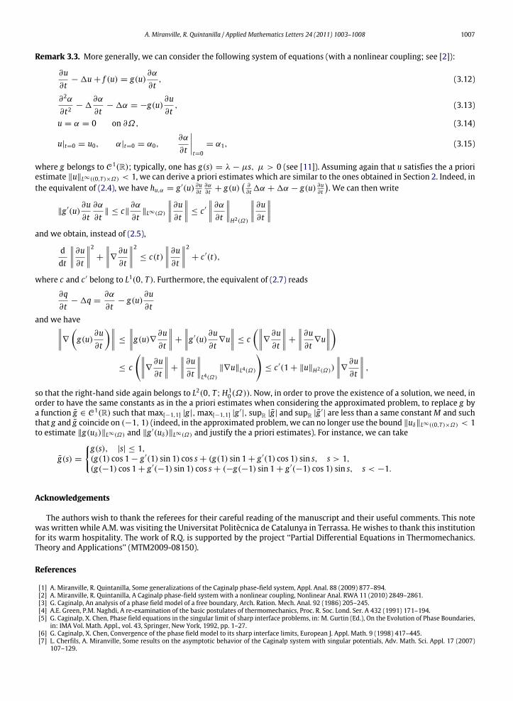
Remark 3.3. More generally, we can consider the following system of equations (with a nonlinear coupling; see [2]):

∂u∂t

− 1u + f (u) = g(u)∂α

∂t, (3.12)

∂2α

∂t2− 1

∂α

∂t− 1α = −g(u)

∂u∂t

, (3.13)

u = α = 0 on ∂Ω, (3.14)

u|t=0 = u0, α|t=0 = α0,∂α

∂t

t=0

= α1, (3.15)

where g belongs to C1(R); typically, one has g(s) = λ − µs, µ > 0 (see [11]). Assuming again that u satisfies the a prioriestimate ‖u‖L∞((0,T )×Ω) < 1, we can derive a priori estimates which are similar to the ones obtained in Section 2. Indeed, inthe equivalent of (2.4), we have hu,α = g ′(u) ∂u

∂t∂α∂t + g(u)

∂∂t 1α + 1α − g(u) ∂u

∂t

. We can then write

‖g ′(u)∂u∂t

∂α

∂t‖ ≤ c‖

∂α

∂t‖L∞(Ω)

∂u∂t

≤ c ′

∂α

∂t

H2(Ω)

∂u∂t

and we obtain, instead of (2.5),

ddt

∂u∂t

2 +

∇ ∂u∂t

2 ≤ c(t)∂u

∂t

2 + c ′(t),

where c and c ′ belong to L1(0, T ). Furthermore, the equivalent of (2.7) reads

∂q∂t

− 1q =∂α

∂t− g(u)

∂u∂t

and we have∇ g(u) ∂u∂t ≤

g(u)∇ ∂u∂t

+

g ′(u)∂u∂t

∇u ≤ c

∇ ∂u∂t

+

∂u∂t

∇u

≤ c

∇ ∂u∂t

+

∂u∂t

L4(Ω)

‖∇u‖L4(Ω)

≤ c ′(1 + ‖u‖H2(Ω))

∇ ∂u∂t

,

so that the right-hand side again belongs to L2(0, T ;H10 (Ω)). Now, in order to prove the existence of a solution, we need, in

order to have the same constants as in the a priori estimates when considering the approximated problem, to replace g bya function g ∈ C1(R) such that max[−1,1] |g|,max[−1,1] |g ′

|, supR |g| and supR |g ′| are less than a same constantM and such

that g and g coincide on (−1, 1) (indeed, in the approximated problem, we can no longer use the bound ‖uδ‖L∞((0,T )×Ω) < 1to estimate ‖g(uδ)‖L∞(Ω) and ‖g ′(uδ)‖L∞(Ω) and justify the a priori estimates). For instance, we can take

g(s) =

g(s), |s| ≤ 1,(g(1) cos 1 − g ′(1) sin 1) cos s + (g(1) sin 1 + g ′(1) cos 1) sin s, s > 1,(g(−1) cos 1 + g ′(−1) sin 1) cos s + (−g(−1) sin 1 + g ′(−1) cos 1) sin s, s < −1.

Acknowledgements

The authors wish to thank the referees for their careful reading of the manuscript and their useful comments. This notewas written while A.M. was visiting the Universitat Politècnica de Catalunya in Terrassa. He wishes to thank this institutionfor its warm hospitality. The work of R.Q. is supported by the project ‘‘Partial Differential Equations in Thermomechanics.Theory and Applications’’ (MTM2009-08150).

References

[1] A. Miranville, R. Quintanilla, Some generalizations of the Caginalp phase-field system, Appl. Anal. 88 (2009) 877–894.[2] A. Miranville, R. Quintanilla, A Caginalp phase-field system with a nonlinear coupling, Nonlinear Anal. RWA 11 (2010) 2849–2861.[3] G. Caginalp, An analysis of a phase field model of a free boundary, Arch. Ration. Mech. Anal. 92 (1986) 205–245.[4] A.E. Green, P.M. Naghdi, A re-examination of the basic postulates of thermomechanics, Proc. R. Soc. Lond. Ser. A 432 (1991) 171–194.[5] G. Caginalp, X. Chen, Phase field equations in the singular limit of sharp interface problems, in: M. Gurtin (Ed.), On the Evolution of Phase Boundaries,

in: IMA Vol. Math. Appl., vol. 43, Springer, New York, 1992, pp. 1–27.[6] G. Caginalp, X. Chen, Convergence of the phase field model to its sharp interface limits, European J. Appl. Math. 9 (1998) 417–445.[7] L. Cherfils, A. Miranville, Some results on the asymptotic behavior of the Caginalp system with singular potentials, Adv. Math. Sci. Appl. 17 (2007)

107–129.

1008 A. Miranville, R. Quintanilla / Applied Mathematics Letters 24 (2011) 1003–1008

[8] L. Cherfils, A. Miranville, On the Caginalp system with dynamic boundary conditions and singular potentials, Appl. Math. 54 (2009) 89–115.[9] M. Grasselli, A. Miranville, V. Pata, S. Zelik, Well-posedness and long time behavior of a parabolic–hyperbolic phase-field system with singular

potentials, Math. Nachr. 280 (2007) 1475–1509.[10] M. Grasselli, H. Petzeltová, G. Schimperna, Long time behavior of solutions to the Caginalp systemwith singular potential, Z. Anal. Anwend. 25 (2006)

51–72.[11] M. Brokate, J. Sprekels, Hysteresis and Phase Transitions, Springer, New York, 1996.