Embed Size (px)
Citation preview
Ann. Inst. Henri Poincaré,
Vol. 35, n◦ 4, 1999, p. 531-572. Probabilités et Statistiques
Abel transform and integrals of Bessel local timesby
Mihai GRADINARU a,1, Bernard ROYNETTE a,Pierre VALLOIS a, Marc YOR b
a Institut de Mathématiques Elie Cartan, Université Henri Poincaré, B.P. 239,54506 Vandœuvre-lès-Nancy Cedex, France
b Laboratoire de Probabilités, Université Pierre et Marie Curie, Tour 56 (3ème étage),4, place Jussieu, 75252 Paris Cedex, France
Manuscript received on 10 June 1998, revised 26 February 1999
ABSTRACT. – We study integrals of the type∫ t
0 ϕ(s) d Ls, whereϕ is apositive locally bounded Borel function and Lt denotes the local time atlevel 0 of a Bessel process of dimensiond, 0< d < 2. Elsevier, Paris
Key words:Bessel local time, Abel’s integral operator
AMS classification: 60J65, 60J55, 45E10
RÉSUMÉ. – Nous étudions les intégrales du type∫ t
0 ϕ(s) d Ls, où ϕest une fonction borelienne positive localement bornée et où Lt est letemps local en 0 d’un processus de Bessel de dimensiond, 0< d < 2. Elsevier, Paris
Mots Clés:Transformée d’Abel et intégrales du temps local de processus de Bessel
1 E-mail: [email protected].
Annales de l’Institut Henri Poincaré- Probabilités et Statistiques - 0246-0203Vol. 35/99/04/ Elsevier, Paris
532 M. GRADINARU ET AL.
INTRODUCTION
Let (Xt, t > 0) be a nice real-valued diffusion, with scale functionsand speed measurem; we are particularly interested in the case whenXtis Brownian motion, or a Bessel process with dimensiond ∈]0,2[.
In a number of problems, the laws of inhomogeneous functionals
t∫0
f (s,Xs) ds
are of interest (see, e.g., [3,4,23]). Such functionals may be representedas (inhomogeneous) integrals of the local times ofX:
t∫0
f (s,Xs) ds =∞∫
0
m(dx)
t∫0
ds Lxs f (s, x), (0.1)
where
Lxt = limε↓0(1/m(x, x + ε)) t∫
0
ds1I{x6Xs6x+ε}
are the (diffusion) local times at levelx associated withX (see, e.g., [11],p. 174).
Although the computations of the laws of∫ t
0 f (s,Xs) ds may beobtained, in theory, from the Feynman–Kac formula, these computationsare not easy in practice. Thus, it seemed natural to first consider the“simplest” cases (in view of (0.1)), i.e., the computations of the laws of
L(ϕ)t :=t∫
0
ϕ(s) d Ls,
where Lt := L0t is the local time at level 0.
Now, the moments of L(ϕ)t are easily obtained in terms of the densitiesp.t (x, y) of the semi-groupPt(x, dy) with respect tom(dy), i.e.:
Pt(x, dy)= p.t (x, y)m(dy).Indeed, it follows from (0.1) and the continuity ofp.t (x, y) (see,again, [11], p. 175), that:
Annales de l’Institut Henri Poincaré- Probabilités et Statistiques
ABEL TRANSFORM AND LOCAL TIMES 533
Ex[dt L
yt
]= p.t (x, y) dt.We denote, for simplicity,q(t) := p.t (0,0). With the help of the Markovproperty, the moments of L(ϕ)t are given by:
E0[(
L(ϕ)t)m]= (m!)E[ t∫
0
t∫s1
· · ·t∫
sm−1
ds1 Ls1 · · ·dsm Lsmϕ(s1) · · ·ϕ(sm)]
= (m!)t∫
0
t∫s1
· · ·t∫
sm−1
ds1ds2 · · ·dsm
× q(s1)q(s2− s1) · · ·q(sm − sm−1)ϕ(s1) · · ·ϕ(sm).Using Fubini’s theorem, we can write:
E0[(
L(ϕ)t)m]= (m!)Qt
(ϕQ•(ϕQ•(· · ·Q•(ϕ 1) · · ·))), (0.2)
where
Qt(ψ) := (Qψ)(t)=t∫
0
q(t − s)ψ(s) ds. (0.3)
In the particular case whenX is the Bessel process with dimensiond = 2(1+ n), wheren∈]−1,0[, we get
q(t)= knt−n−1, kn := 2−n0(n+ 1)−1, (0.4)
so thatQ is then a multiple of the Abel integral operator (see Section 1.5below) with index α = −n. Hence, the Abel integral operators arenaturally closely related to the laws of L(ϕ)t for Bessel processes (see alsoRemark 4.1).
More generally, the above computations, which could be extended tothe computations of the moments of
∫ t0 f (s,Xs) ds are well-understood
in the diffusion literature (see, e.g., [19] for some particular examples).However, what may be a little newer is that in this paper is our
characterization of the law of
L(ϕ)t (R) :=t∫
0
ϕ(s) d Ls(R)
for the Bessel processR, for the Bessel bridge, conditioned to take thevaluey in time 1, and in particulary = 0. Recall that L(1)1 (R)= L1(R) is
Vol. 35, n◦ 4-1999.
534 M. GRADINARU ET AL.
a Mittag-Leffler random variable with parameter|n| (see, e.g., [7], p. 447or [14], p. 129).
Moreover, we show that the random variables
RZ and
Z∫0
ϕ(1−Z+ v) d Lv(R) (0.5)
are independent, and∫ Z
0 ϕ(1−Z+v) d Lv(R) is exponentially distributedwith parameter 1. Here,Z is a random variable independent fromR. Itsprobability density function,αf on [0,1], is the Abel transform of index1+ n of the derivative of a regular increasing functionf . The functionϕis related tof by the equalityϕ = αf /f .
Clearly, the particular casen=−1/2 corresponds to the process|B|,with B the linear Brownian motion.
Our approach is based on two probabilistic representations for the so-lution of a partial differential equation with mixed boundary conditions.Using Abel’s transform and these two representations (the backward Kol-mogorov representation and the Fokker–Planck representation) we de-duce some useful information on functionals of local time L(ϕ)
t . Someresults obtained here may be proved using the dual predictable projectionof the last passage time in 0 (see another proof of Corollary 3.4).
The plan of the paper is as follows. After some useful preliminaries onBessel processes and Abel operators (Section 1), we give the probabilisticrepresentations for the solution of this partial differential equation and theanalytic relations involving Abel’s transform (Section 2). In Section 3we state our main results. The proofs are given in Section 4. Wealso make a number of remarks. This paper is a complement and ageneralization of [10]. One of the novelties in this paper is the importanceof the Abel transform which we had not realized, hence also notintroduced in our 1997 preprint. Finally, for practical and pedagogicalpurposes, we collect in Appendix A the main formulas obtained in bothpapers.
1. PRELIMINARIES
In this section we review a few basic facts on Bessel processes and onAbel operators. For the proofs of these results, the reader may consult thebook [17], Chapter XI (see, also, for a number of applications, [15,20,22]), respectively, the book [9], Chapter 4.
Annales de l’Institut Henri Poincaré- Probabilités et Statistiques
ABEL TRANSFORM AND LOCAL TIMES 535
1.1. Bessel processes and Bessel semi-groups
For anyd > 0 we denote byR2t the square of ad-dimensional Bessel
process, the unique solution of the stochastic differential equation
R2t =R2
0 + 2
t∫0
√R2s dβs + d t,
whereβ is a linear Brownian motion. The law of the square of ad-di-mensional Bessel process, started atx, is denotedQ(d)
x and satisfies thefollowing additivity property:
Q(d)x ∗Q(d ′)
x ′ =Q(d+d ′)x+x ′ ,
for everyd, d ′ > 0 andx, x′ > 0. Take 0< d < 2 and denote byn :=d/2− 1∈]−1,0[ the index of the Bessel process, andQn
x :=Q(d)x . From
the additivity property we deduce the Laplace transform
EQnx[exp(−λR2
t
)]= (1+ 2λ t)−(n+1) exp(−λx/(1+ 2λt)
).
By inverting the Laplace transform we get, forn >−1, the density of thesemi-group of the square of the Bessel process of indexn, started atx:
qnt (x, y) := (2t)−1(y/x)n/2 exp(−(x + y)/2t) In(
√xy/t),
t > 0, x > 0,
where In is the Bessel function of indexn. For x = 0 this densitybecomes:
qnt (0, y) := (2t)−n−10(n+ 1)−1yn e−y/2t .
The square root of the square of a Bessel process of indexn, started ata2,Rt , is called the Bessel process of indexn started ata > 0. Its law willbe denoted by Pna. The density of the semi-group is obtained from that ofthe square of a Bessel process of indexn, by a straightforward change ofvariable. We obtain, forn >−1,
pnt (x, y) := (y/t)(y/x)n exp(−(x2+ y2)/2t
)In(xy/t),
t, x > 0, (1.1)
and
pnt (0, y) := 2−n0(n+ 1)−1t−n−1y2n+1 e−y2/2t , y > 0. (1.1′)
Vol. 35, n◦ 4-1999.
536 M. GRADINARU ET AL.
From (1.1) we see that, for positive Borel functionsu, v,⟨Πnt u, v
⟩ν= ⟨u,Πn
t v⟩ν, t > 0, (1.2)
whereΠnt denotes the semi-group of the Bessel process of indexn
Πnt u(a) := Ena
[u(Rt)
],
and
〈u, v〉ν :=∞∫
0
u(x)v(x)x2n+1 dx.
Hence the semi-group is symmetric with respect to the invariant measuregiven by:
ν(dx) := x2n+11I]0,∞[(x) dx. (1.2′)
The infinitesimal generator of the Bessel process is
L= (1/2)(∂2/∂x2)+ ((2n+ 1)/2x)(∂/∂x) (1.3)
on
D(L) :={f : f, Lf ∈Cb([0,∞[), lim
x↓0 x2n+1f ′(x)= 0
}(1.3′)
(see also [13], p. 761, or [6], pp. 114–115).A continuous process(rt : t ∈ [0, t0]), the law of which is equal to
Pn,t0a,b (·) := Pna(· |Rt0 = b)
is called the Bessel bridge froma to b over[0, t0]. In the sequel, we shallbe interested in the Bessel bridgert from 0 to 0 over[0,1− s], withs ∈ [0,1].1.2. Absolute continuity properties and law of the first hitting time
of 0
It is known that for−1<n< 0 the point 0 is reached a.s. under Pnx and
it is instantaneously reflecting. Let us denoteT0 := inf{t > 0: Rt = 0}andFt := σ {Rs: s 6 t}. Then, the laws of the Bessel processes satisfy
Annales de l’Institut Henri Poincaré- Probabilités et Statistiques
ABEL TRANSFORM AND LOCAL TIMES 537
the following absolute continuity property:
(Pna)|Ft∩{t<T0} = (Rt/a)n exp
(−(n2/2)
t∫0
ds/R2s
)· (P0
a
)|Ft ,
an equality which is satisfied for everyn>−1. Note that P0a is the law ofthe 2-dimensional Bessel process starting froma. From this we deduce,for −16 n < 0, (
Pna)|Ft∩{t<T0} = (a/Rt)2|n| ·
(P|n|a)|Ft , (1.4)
(|n| = −n, since−16 n < 0).Let us denote byΠ
n
t the semi-group of the Bessel process killed atT0
Πn
t u(x) := Enx[u(Rt)1I{t<T0}
],
and we can deduce from (1.2) and (1.4), that, for positive Borel functionsu, v, ⟨
Πn
t u, v⟩ν= ⟨u,Π n
t v⟩ν, t > 0. (1.5)
Moreover, by (1.4), we can deduce the Williams’ time-reversal prop-erty: the processes
{RT0−t : t < T0} under Pnx and{Rt : t < γx} under P|n|0 (1.6)
are identical in law (cf. [18], p. 1158 or [15], p. 302). Here we denote
γx := sup{t : Rt = x}.Therefore
Pnx(T0 ∈ dt)= P|n|0 (γx ∈ dt).Using a result in [15], p. 329 (or [17], p. 308, Ex. (4.16), 5◦), we can write
P|n|0 (γx ∈ dt)= (|n|/x)p|n|t (0, x) dt.
Using (1.1′) we obtain the density ofT0, under Pnx ,
φ(x, t) := (d/dt)Pnx(T06 t)= 2n0(|n|)−1tn−1x−2n e−x
2/2t , x, t > 0 (1.7)
(for this particular result andn> 1/2, see also [8], p. 864).
Vol. 35, n◦ 4-1999.
538 M. GRADINARU ET AL.
We also note that, using the strong Markov property atT0 we get, fory > 0,
pn,νt (0, y)= pn,νt (y,0)=t∫
0
φ(y, s)pn,νt−s (0,0) ds. (1.8)
Herepn,νt (0, y) is the density of the semi-groupΠnt with respect to the
invariant measureν.
1.3. Local time at level 0
The local time at levelx for the Bessel process Lxt (R) can be definedas an occupation density: for every positive Borel functionh,
t∫0
h(Rs) ds = 2
∞∫0
h(x)Lxt (R)x2n+1dx. (1.9)
Note that we use a different normalisation than in the formula in [17],p. 308, Ex. (4.16), 4◦ and also than in (0.1) in the Introduction.
This choice of local times agrees with the fact thatR2|n|t −2|n|L0
t (R) isa martingale. Indeed,R2|n|
t is aFt -submartingale and it suffices to writeits Doob–Meyer decomposition to obtain L0
t (R) (up to a constant factor).We often denote Lt (R) instead of L0t (R).
Let us now mention two related scaling properties. Firstly, the Besselprocess has the Brownian scaling property, that is, for any realc > 0,the processesRc t andc1/2Rt have the same law, whenR0= 0. Secondly,{Lt (R): t > 0} inherits fromR the following scaling property: indeed,by (1.9), {
Lc t (R): t > 0} (law)= {
c|n| Lt (R): t > 0}. (1.10)
We also recall that,
1∫0
ϕ(t)d Lt (R) <∞⇔1∫
0
ϕ(t)t−n−1 dt <∞ (1.11)
(see [16], p. 655, and [12], p. 44, for the case of Brownian motion,n=−1/2).
Annales de l’Institut Henri Poincaré- Probabilités et Statistiques
ABEL TRANSFORM AND LOCAL TIMES 539
1.4. A simple path decomposition and the Bessel meander
It is known that, conditionally ongt , {Rs: s 6 gt} is independent of{Rs: s > gt }, wheregt := sup{s 6 t : Rs = 0}. More precisely, the Besselmeander
mt(u) := (1/√t − gt )Rgt+u(t−gt ), u ∈ [0,1], (1.12)
is independent ofFgt (see [20], p. 42). Let us recall also that, for fixedt > 0,
gt(law)= tZ−n,1+n,
where byZa,b we denote a beta random variable with parametersa, b
> 0:
P(Za,b ∈ du)= B(a, b)−1ua−1(1− u)b−11I]0,1[(u) du.Moreover, for everyt > 0,
mt(1)=Rt/√t − gt (law)= √2E(1), (1.2′)
whereE(1) denotes an exponential variable with parameter 1 and√
2E(1)is a Rayleigh random variable having densityue−u2/21I[0,∞[(u).
1.5. Abel’s integral operator
The Abel transform of a positive Borel functionf on [0,∞[, is definedas
J αf (t) := 0(α)−1
t∫0
(t − u)α−1f (u) du, t > 0, (1.13)
where α > 0. The operatorJ α is called Abel integral operator, orfractional integral operator. Our principal interest is for 0< α 6 1.Clearly, J 1 is the ordinary integration operator, that isJ 1f is theprimitive of f .
By straightforward calculation we can verify that, forα,β > 0,
J α ◦ J β = J α+β. (1.14)
This, together with the previous remark, implies, iff (0)= 0,
J α+1(f ′)= J αf. (1.14′)
Vol. 35, n◦ 4-1999.
540 M. GRADINARU ET AL.
Let us also note that ifεγ (t) := tγ , γ >−1, then
J αεγ = (0(γ + 1)/0(α+ γ + 1))εα+γ . (1.15)
2. TWO PROBABILISTIC REPRESENTATIONS
Let us considerω0 a continuous function with growth less thanexponential at infinity, andf a continuous function such thatf ∈C1(]0,∞[). Assume thatω0(0)= f (0)= 0.
2.1. Dirichlet and Fokker–Planck representations
Recall thatL is the generator of the Bessel process (see (1.3)). Thereis existence and uniqueness of the solution of the problem
(∂ω/∂t) (t, x)= (Lω)(t, x), t, x > 0, (2.1)
with
ω(0, x)=ω0(x), x > 0, (2.2)
and
ω(t,0)= f (t), t > 0. (2.3)
It admits both a Dirichlet representation (Proposition 2.1 below) anda Fokker–Planck representation (Proposition 2.2 below). We shall thencompare these two representations (Proposition 2.3 below).
PROPOSITION 2.1. –The solutionω(t, x) of (2.1)–(2.3)can be writ-ten as
ω(t, x)= ω1(t, x)+ω2(t, x), t, x > 0, (2.4)
where
ω1(t, x) := Enx[ω0(Rt)1I{t<T0}
], t, x > 0, (2.5)
ω2(t, x) := Enx[f (t − T0)1I{t>T0}
]= t∫0
φ(x, s)f (t − s) ds,
t > 0, x > 0. (2.6)
Proof. –To obtain (2.4) it suffices to solve the Dirichlet problem for theoperatorL− ∂/∂t on [0,∞[×[0, t] (see also[10], Proposition 1.2).2
Annales de l’Institut Henri Poincaré- Probabilités et Statistiques
ABEL TRANSFORM AND LOCAL TIMES 541
PROPOSITION 2.2. –The solutionω(t, x) of (2.1)–(2.3) (also) admitsthe following Fokker–Planck representation
y2n+1ω(t, y)
=∞∫
0
ω0(x)pnt (x, y)x
2n+1 dxEnx
[exp
(−
t∫0
ϕ(s) d Ls(R)
)|Rt = y
],
t, y > 0, (2.7)
where, ifω is given by(2.4),
ϕ(t) := (1/f (t)) limx↓0 x
2n+1(∂ω/∂x) (t, x), t > 0. (2.8)
Remark. – (i) Unlike formulae (2.5) and (2.6), formula (2.7) featuresthe “unknown” functionω both on its left and right hand sides.
(ii) The decomposition (2.4),ω = ω1 + ω2 yields a correspondingdecomposition
ϕ = ϕ1+ ϕ2
(with obvious notation). In Proposition 2.4 below,f ϕ1 andf ϕ2 shall begiven in a closed form, in terms, respectively, ofω0 andf .
Proof of Proposition 2.2. –Let ϕ be given by (2.8) and define
Mt := exp
(−
t∫0
ϕ(s) d Ls(R)
).
We introduce, fort > 0, x > 0, the functionω(t, x) defined by⟨h(·), ω(t, ·)⟩
ν:= Enω0ν
[h(Rt)Mt
]. (a)
Hereh is an arbitrary bounded positive Borel function and we denote
Pnω0ν(A) :=
∞∫0
Pnx(A)ω0(x)x2n+1 dx.
(i) Let g : [0,∞[×[0,∞[→ [0,∞[ be a smooth function with compactsupport disjoint of[0,∞[×{0}. Ito’s formula gives
Vol. 35, n◦ 4-1999.
542 M. GRADINARU ET AL.
g(t,Rt)Mt = g(0, x)+t∫
0
(∂g/∂x)(s,Rs)Ms dBs
+t∫
0
(∂g/∂s +Lg)(s,Rs)Ms ds,
so, taking the expectation, we can write⟨g(t, ·), ω(t, ·)⟩
ν= ⟨g(0, ·),ω0(·)⟩ν+
t∫0
⟨(∂g/∂s +Lg)(s, ·), ω(s, ·)⟩
νds.
Taking the derivative with respect tot we get⟨g(t, ·), (∂ω/∂t)(t, ·)⟩
ν= ⟨(Lg)(t, ·), ω(t, ·)⟩
ν. (b)
Since the support ofg is disjoint of [0,∞[×{0}, integrating by parts wededuce ⟨
g(t, ·), (∂ω/∂t)(t, ·)⟩ν= ⟨g(t, ·), (Lω)(t, ·)⟩
ν.
Henceω satisfies (2.1).(ii) Let us consideru and v two smooth functions defined on[0,∞[and take nowg : [0,∞[×[0,∞[→ R a smooth function with compactsupport such thatg(t, x) := u(t)x2|n| + v(t) in a neighbourhood of[0,∞[×{0}. SinceR2|n|
t −2|n|Lt (R) is a martingale, Ito’s formula gives
g(t,Rt)Mt = g(0, x)+t∫
0
(∂g/∂x)(s,Rs)Ms dBs
+t∫
0
Lg(s,Rs)Ms ds +t∫
0
(∂g/∂s)(s,Rs)Ms ds
+t∫
0
(2|n|u(s)− ϕ(s)v(s))Ms d Ls(R).
(iii) Assume thatu, v,ϕ verify
2|n|u(s)− ϕ(s) v(s)= 0. (c)
By the same arguments of (i) and by (c), we obtain again (b). Since theassumptions on the functiong are different, let us detail the integration
Annales de l’Institut Henri Poincaré- Probabilités et Statistiques
ABEL TRANSFORM AND LOCAL TIMES 543
by parts on the right hand of (b). Using the form (1.3) of the operatorLwe can write,⟨(Lg)(t, ·), ω(t, ·)⟩
ν
=(
1
2
∂g
∂x(t, x)x2n+1ω(t, x)
)x↑∞x↓0− 1
2
∞∫0
∂g
∂x(t, x)x2n+1 ∂ω
∂x(t, x) dx
=(
1
2
∂g
∂x(t, x)x2n+1ω(t, x)
)x↓0−(
1
2g(t, x)x2n+1∂ω
∂x(t, x)
)x↑∞x↓0
+ 1
2
∞∫0
g(t, x)∂
∂x
(x2n+1∂ω
∂x(t, x)
)dx
= |n|u(t)ω(t,0)− v(t)2
limx↓0 x
2n+1∂ω
∂x(t, x)+ ⟨g(t, ·), (Lω)(t, ·)⟩
ν.
Sinceω verifies (2.1), replacing the above equality in (b), we deduce
2|n|u(t)ω(t,0)− v(t) limx↓0 x
2n+1(∂ω/∂x)(t, x)= 0. (d)
(iv) Sinceu, v are arbitrary functions, combining (c) and (d) we get
limx↓0 x
2n+1∂ω
∂x(t, x)− ω(t,0)
ω(t,0)limx↓0 x
2n+1∂ω
∂x(t, x)= 0. (e)
Moreover,ω satisfies
ω(0, x)= ω0(x), ∀x > 0.
Sinceω andω verify the same parabolic equation (2.1) with the sameinitial and mixed boundary conditions (2.2) and (2.3), we deduce thatω= ω.(v) Therefore, by (a) we deduce that, for every bounded positive Borelfunctionh,
∞∫0
h(y)ω(t, y)y2n+1 dy
=∞∫
0
ω0(x)x2n+1 dx Enx
[h(Rt)exp
(−
t∫0
ϕ(s) d Ls(R)
)].
Vol. 35, n◦ 4-1999.
544 M. GRADINARU ET AL.
By conditioning with respect toRt = y on the right hand side of the aboveequality we obtain (2.7), sinceh is arbitrary. 2
Now, the Dirichlet representation ofω naturally decomposesω intoω1+ω2 and, in the next proposition, we also find this decomposed formin the Fokker–Planck representation.
PROPOSITION 2.3. –The decompositionω = ω1 + ω2 appears asfollows in the Fokker–Planck representation: for t, y > 0,
y2n+1ω1(t, y)=∞∫
0
ω0(x)pnt (x, y)x
2n+1 dx Pnx[T0> t |Rt = y]
= y2n
∞∫0
ω0(x)p|n|t (x, y)x dx, (2.9)
and
y2n+1ω2(t, y)=∞∫
0
ω0(x)pnt (x, y)x
2n+1 dx
×Enx
[exp
(−
t∫0
ϕ(s)d Ls(R)
)1I{t>T0}
∣∣∣Rt = y], (2.10)
or, equivalently,
y2n+1ω2(t, y)=t∫
0
dsEn0
[exp
(−
t−s∫0
ϕ(s + v) d Lv(R)
)∣∣∣Rt−s = y]
×∞∫
0
x2n+1ω0(x)φ(x, s)pnt−s (0, y) dx, t, y > 0. (2.11)
Here,pnt is given by(1.1), (1.1′), φ by (1.7)andϕ by (2.8).
Proof. –The first equality in (2.9) is only the translation of thesymmetry of the semi-group of the killed Bessel processΠ
n
t , with respectto the measureν (see (1.5)). The second equality in (2.9) is obtainedthanks to formulae (1.1) and (1.4), from which the formula
Pnx(T0> t |Rt = y)= (I|n|/In)(xy/t)follows. To get (2.11) we use the strong Markov property atT0. 2
Annales de l’Institut Henri Poincaré- Probabilités et Statistiques
ABEL TRANSFORM AND LOCAL TIMES 545
2.2. Analytic relations involving Abel’s transform
There exist some analytic relations between the functionsω0, f andϕinvolving Abel’s transform (cf. Proposition 2.4 below).
Recall thatf is a continuous function such thatf ∈ C1(]0,∞[) andf (0)= 0. Let us introduce, fort > 0, and−1< n< 0, the constant
cn := 2n+10(n+ 1)/0(|n|), (2.12)
and the function
αf (t) := cn(J n+1f ′)(t). (2.12′)
Recall that, from (1.14′), we have(J 1αf )(t)= cn(J n+1f )(t), hence
kf :=1∫
0
αf (t) dt = cn(J n+1f)(1). (2.13)
We now give the promised explicit representations ofϕ1 andϕ2 (seethe remark following Proposition 2.2):
PROPOSITION 2.4. –Assume thatϕ is given by (2.8) with ω thesolution of(2.1)–(2.3). Writeϕ = ϕ1+ ϕ2, where
ϕi(t) := (1/f (t)) limx↓0 x
2n+1(∂ωi/∂x)(t, x), i = 1,2. (2.8′)
Then, we have
(ϕ1f )(t)= (2n+1/0(|n|))tn−1
∞∫0
yω0(y)e−y2/2tdy, t > 0, (2.14)
(ϕ2f )(t)=−αf (t), t > 0, (2.15)
and, consequently:
(αf + ϕf )(t)= (2n+1/0(|n|))tn−1
∞∫0
yω0(y)e−y2/2t dy, t > 0. (2.16)
Proof. –We need to compute the limits in (2.8′). First, using (2.9)and (1.1), we can write
Vol. 35, n◦ 4-1999.
546 M. GRADINARU ET AL.
ω1(t, x)= (1/(txn)) ∞∫0
yn+1ω0(y)exp(−(x2+ y2)/2t
)I|n|(xy/t) dy. (a)
Since
I|n|(y)∼ (y/2)|n|
0(|n| + 1), I′|n|(y)∼
(y/2)|n|−1
20(|n|) , asy ∼ 0,
(2.14) follows from (a) by direct calculation.On the other hand, by (2.6) and (1.7), we can write
x2n(ω2(t, x)−ω2(t,0))
= (2n/0(|n|))( t∫0
sn−1 e−x2/2s(f (t − s)− f (t))ds
− f (t)∞∫t
sn−1 e−x2/2s ds
),
from which we deduce(2|n|)−1
(ϕ2f )(t)
= (2n/0(|n|))( t∫0
sn−1(f (t − s)− f (t))ds + tnf (t)/n). (b)
To obtain (2.15), we write in (b),f (t − s)− f (t) = ∫ t−st f ′(u) du, and,by straighforward calculation, we find (2.12′). 2
3. MAIN RESULTS
Before stating our new results, we explain the guiding idea behindthem: supposeω0 andf are given. We shall write another form of (2.11),using (2.6) and (2.16). Fort = 1 and everyy > 0, we get
y
1∫0
(2n+1/0(|n|))sn−1 e−y
2/2sf (1− s) ds
=1∫
0
(αf + ϕf )(s)pn1−s(0, y) ds
×En0
[exp
(−
1−s∫0
ϕ(s + v) d Lv(R)
)∣∣∣R1−s = y],
Annales de l’Institut Henri Poincaré- Probabilités et Statistiques
ABEL TRANSFORM AND LOCAL TIMES 547
since, by (1.7),
x2n+1ω0(x)φ(x, s)= 2n0(|n|)−1xω0(x)sn−1 e−x
2/2s.
The first above equality was obtained using the two probabilisticrepresentations (2.1)–(2.3) and Abel’s transform. We see that the givenfunction ω0 does not appear in the above equality. It suggests thefollowing general result, where, this timef and ϕ are given as newparameters:
THEOREM 3.1. –Consider the continuous functionsf : [0,1] →[0,∞[ and ϕ : ]0,1] → [0,∞[. Assume thatf ∈ C1(]0,1]), f (0) = 0and thatt |n|ϕ(t) converges ast ↓ 0. If αf is given by(2.12′), then, foreveryy > 0,
1∫0
(αf + ϕf )(1− s)pns (0, y) ds
×En0
[exp
(−
s∫0
ϕ(1− s + v) d Lv(R)
)∣∣∣Rs = y]
= (2n+1/0(|n|))y 1∫0
sn−1 e−y2/2sf (1− s) ds (3.1)
or, equivalently, for any positive bounded Borel functionh,
1∫0
(αf + ϕf )(1− s) dsEn0[h(Rs)exp
(−
s∫0
ϕ(1− s + v) d Lv(R)
)]
= (2n+1/0(|n|)) ∞∫0
yh(y) dy
1∫0
sn−1 e−y2/2sf (1− s) ds. (3.1′)
In Remark 4.13 we prove a reciprocal result to Theorem 3.1. Asconsequences of this theorem, we can prove the following interestingresults: Propositions 3.2 and 3.3 below concern the Bessel process,whereas Propositions 3.5 and 3.6 below concern the Bessel bridger (seealso the end of the Section 1.1).
PROPOSITION 3.2. –Consider a continuous increasing functionf : [0,1] → [0,∞[ such thatf ∈ C1(]0,1]), f (0) = 0 and f ′(t) ∼ ctp(for some constantsc,p > 0) as t ↓ 0. We also assume, without lossof generality, that the functionf is chosen such that the constantkf
Vol. 35, n◦ 4-1999.
548 M. GRADINARU ET AL.
in (2.13) equals 1. Consider a random variableZ with the proba-bility density functionαf (1− s)1I[0,1](s), independent ofR. Then, forϕ := αf /f , the random variables
RZ and
Z∫0
ϕ(1−Z + v) d Lv(R) (3.2)
are independent. Moreover,
Z∫0
ϕ(1−Z+ v) d Lv(R)(law)= E(1). (3.3)
PROPOSITION 3.3. –Consider a continuous functionϕ : ]0,1]→ [0,∞[ such thatt |n|ϕ(t) converges ast ↓ 0. For λ > 0, we denote
Λϕ(a) := En0
[exp
(−λ
1−a∫0
ϕ(a + v) d Lv(R)
)], a ∈ [0,1]. (3.4)
Then, (I + (λ/cn)Aϕ)Λϕ = 1, (3.5)
where, cn is given by (2.12), and we denote, for a positive Borelfunctionh,
(Aϕh)(a) := J−n(ϕh )(1− a), a ∈ [0,1]. (3.6)
Here and elsewhereh(a) := h(1− a). Hence,
Λϕ(a)=∑k>0
(−λ/cn)k(Akϕ1)(a), a ∈ [0,1]. (3.7)
COROLLARY 3.4. –For any random variableZ > 0 a.s., independentofR, the integral
(2n+1/0(|n|)) Z∫
0
(Z − v)n d Lv(R) (3.8)
is a standard exponential variable and is independent ofZ.
In Remark 4.6 we prove a reciprocal result to Corollary 3.4.
Annales de l’Institut Henri Poincaré- Probabilités et Statistiques
ABEL TRANSFORM AND LOCAL TIMES 549
PROPOSITION 3.5. –Consider a continuous increasing functionf :[0,1] → [0,∞[ such thatf ∈ C1(]0,1]), f (0) = 0 and f ′(t) ∼ ctp(for some constantsc,p > 0) as t ↓ 0. We also assume, without lossof generality, that the functionf is chosen such thatf (1) = 1/2, or,equivalently
2−n0(n+ 1)−1
1∫0
(1− t)−n−1αf (t) dt = 1. (3.9)
Consider a random variableZ with the probability density function
2−n0(n+ 1)−1s−n−1αf (1− s)1I[0,1](s),
andZ is independent ofr. Then, forϕ := αf /f ,
Z∫0
ϕ(1−Z + v) d Lv(r)(law)= E(1). (3.10)
COROLLARY 3.6. –If Z(law)= Z|n|,α , α > 0, is a beta random variable,
independent ofr, then,
2n+10(n+ 1)B(|n|, α)−1
Z∫0
(1−Z+ v)n d Lv(r)(law)= E(1). (3.10′)
PROPOSITION 3.7. –Consider a continuous functionϕ : ]0,1] →[0,∞[ such thatt |n|ϕ(t) converges ast ↓ 0. For λ > 0, we denote
Ξϕ(a) := En0
[exp
(−λ
1−a∫0
ϕ(a + v) d Lv(r)
)], a ∈ [0,1]. (3.11)
Then, (I + (λ/cn)Bϕ)Ξϕ = 1, (3.12)
wherecn is given by(2.12), and we denote, for a positive Borel functionh,
(Bϕh)(a) := (1− a)n+1J−n(ϕ ε−n−1 h
)(1− a), a ∈ [0,1] (3.13)
Vol. 35, n◦ 4-1999.
550 M. GRADINARU ET AL.
(recall thatεγ (s)= sγ ). Hence,
Ξϕ(a)=∑k>0
(−λ/cn)k(Bkϕ1)(a), a ∈ [0,1]. (3.14)
4. PROOFS AND REMARKS
Proof of Theorem 3.1. –(i) Let us denoteψ(t) := t |n|ϕ(t). It is enoughto consider (3.1) forf andψ positive polynomials. Indeed, for generalfunctionsf , ψ , the result is obtained by a limiting procedure: there existpositive polynomialsfk andψk, such that
fk→ f, f ′k→ f ′, ψk→ψ,
uniformly, whenk ↑∞ (thusαfk→ αf ).(ii) As said in the beginning of the previous section, to get (3.1) we needto verify the equalities (2.11) (combined with (2.6)) and (2.16). Supposethat, for givenf , ϕ, the integral equation (2.16) has a solution,ω0.Then, Section 2.1 asserts the existence of the solutionω(t, x) of theproblem (2.1)–(2.3), with boundary conditionsf and ω0. Moreover,by (2.8), we can find a function, which we denote, for the moment, asϕ. Since, by Proposition 2.4,ϕ verifies (2.16) we conclude thatϕ = ϕ.Finally, by Propositions 2.1–2.3 we get (2.11). Therefore, we need tostudy the integral equation (2.16).(iii) By composition withJ−n in (2.16), and using (1.14′), and (2.12′),we obtain
0(n+ 1) f (t)+ (0(|n|)/2n+1)J−n(ϕf )(t)= 0(−n)−1
∞∫0
yω0(y) dy
t∫0
(t − u)−n−1un−1 e−y2/2u du (a)
(sincef (0)= 0). Now we use the next equality
t∫0
(t − u)−n−1un−1 e−y2/2u du= 2−n0(−n)t−n−1y2n e−y
2/2t . (b)
We can verify (b), by (1.8), (1.7) and (1.1′). Replacing (b) in (a) and usingagain (1.1′) we obtain that (2.16) is equivalent to
f (t)+ (1/cn)J−n(ϕf )(t)=Πnt ω0(0). (c)
Annales de l’Institut Henri Poincaré- Probabilités et Statistiques
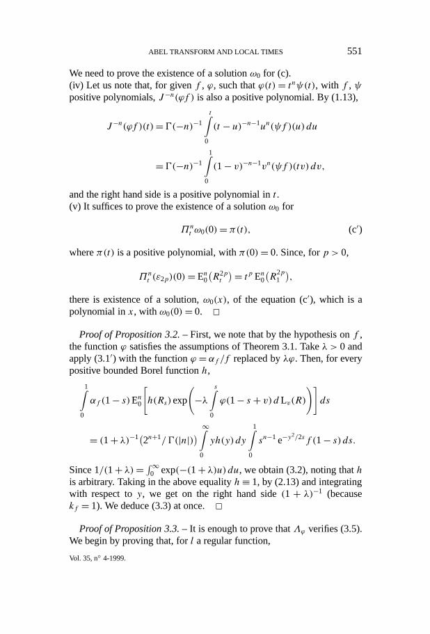
ABEL TRANSFORM AND LOCAL TIMES 551
We need to prove the existence of a solutionω0 for (c).(iv) Let us note that, for givenf , ϕ, such thatϕ(t)= tnψ(t), with f , ψpositive polynomials,J−n(ϕf ) is also a positive polynomial. By (1.13),
J−n(ϕf )(t)=0(−n)−1
t∫0
(t − u)−n−1un(ψf )(u) du
=0(−n)−1
1∫0
(1− v)−n−1vn(ψf )(tv) dv,
and the right hand side is a positive polynomial int .(v) It suffices to prove the existence of a solutionω0 for
Πnt ω0(0)= π(t), (c′)
whereπ(t) is a positive polynomial, withπ(0)= 0. Since, forp > 0,
Πnt (ε2p)(0)=En0
(R2pt
)= tp En0(R
2p1
),
there is existence of a solution,ω0(x), of the equation (c′), which is apolynomial inx, with ω0(0)= 0. 2
Proof of Proposition 3.2. –First, we note that by the hypothesis onf ,the functionϕ satisfies the assumptions of Theorem 3.1. Takeλ > 0 andapply (3.1′) with the functionϕ = αf /f replaced byλϕ. Then, for everypositive bounded Borel functionh,
1∫0
αf (1− s)En0[h(Rs)exp
(−λ
s∫0
ϕ(1− s + v) d Lv(R)
)]ds
= (1+ λ)−1(2n+1/0(|n|)) ∞∫0
yh(y) dy
1∫0
sn−1 e−y2/2sf (1− s) ds.
Since 1/(1+ λ)= ∫∞0 exp(−(1+ λ)u) du, we obtain (3.2), noting thathis arbitrary. Taking in the above equalityh≡ 1, by (2.13) and integratingwith respect toy, we get on the right hand side(1 + λ)−1 (becausekf = 1). We deduce (3.3) at once.2
Proof of Proposition 3.3. –It is enough to prove thatΛϕ verifies (3.5).We begin by proving that, forl a regular function,
Vol. 35, n◦ 4-1999.
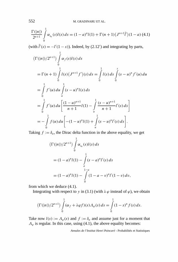
552 M. GRADINARU ET AL.
0(|n|)2n+1
1∫0
αδa(s)l(s) ds = (1− a)nl(1)+ 0(n+ 1)
(J n+1l′
)(1− a) (4.1)
(with l′(s)=−l′(1− s)). Indeed, by (2.12′) and integrating by parts,
(0(|n|)/2n+1) 1∫
0
αf (s)l(s) ds
= 0(n+ 1)
1∫0
l(s)(J n+1f ′
)(s) ds =
1∫0
l(s) ds
s∫0
(s − u)nf ′(u) du
=1∫
0
f ′(u) du1∫u
(s − u)nl(s) ds
=1∫
0
f ′(u) du[(1− u)n+1
n+ 1l(1)−
1∫u
(s − u)n+1
n+ 1l′(s) ds
]
=−1∫
0
f (u) du
[−(1− u)nl(1)+
1∫u
(s − u)nl′(s) ds].
Takingf := δa , the Dirac delta function in the above equality, we get
(0(|n|)/2n+1) 1∫
0
αδa(s)l(s) ds
= (1− a)nl(1)−1∫a
(s − a)nl′(s) ds
= (1− a)nl(1)−1−a∫0
(1− a − v)nl′(1− v) dv,
from which we deduce (4.1).Integrating with respect toy in (3.1) (withλϕ instead ofϕ), we obtain
(0(|n|)/2n+1) 1∫
0
(αf + λϕf )(s)Λϕ(s) ds =1∫
0
(1− s)nf (s) ds.
Take nowl(s) :=Λϕ(s) andf := δa and assume just for a moment thatΛϕ is regular. In this case, using (4.1), the above equality becomes:
Annales de l’Institut Henri Poincaré- Probabilités et Statistiques
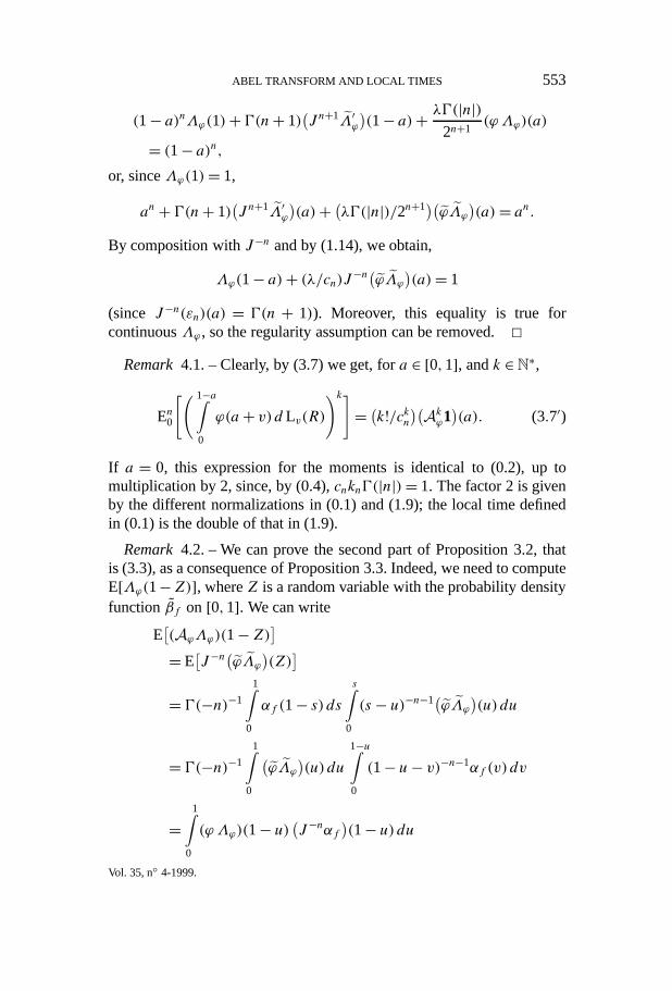
ABEL TRANSFORM AND LOCAL TIMES 553
(1− a)nΛϕ(1)+0(n+ 1)(J n+1Λ′ϕ
)(1− a)+ λ0(|n|)
2n+1(ϕΛϕ)(a)
= (1− a)n,or, sinceΛϕ(1)= 1,
an + 0(n+ 1)(J n+1Λ′ϕ
)(a)+ (λ0(|n|)/2n+1)(ϕΛϕ
)(a)= an.
By composition withJ−n and by (1.14), we obtain,
Λϕ(1− a)+ (λ/cn)J−n(ϕΛϕ
)(a)= 1
(since J−n(εn)(a) = 0(n + 1)). Moreover, this equality is true forcontinuousΛϕ , so the regularity assumption can be removed.2
Remark4.1. – Clearly, by (3.7) we get, fora ∈ [0,1], andk ∈N∗,
En0
[( 1−a∫0
ϕ(a + v) d Lv(R)
)k]= (k!/ckn)(Akϕ1)(a). (3.7′)
If a = 0, this expression for the moments is identical to (0.2), up tomultiplication by 2, since, by (0.4),cnkn0(|n|)= 1. The factor 2 is givenby the different normalizations in (0.1) and (1.9); the local time definedin (0.1) is the double of that in (1.9).
Remark4.2. – We can prove the second part of Proposition 3.2, thatis (3.3), as a consequence of Proposition 3.3. Indeed, we need to computeE[Λϕ(1−Z)], whereZ is a random variable with the probability densityfunction βf on [0,1]. We can write
E[(AϕΛϕ)(1−Z)]= E
[J−n
(ϕΛϕ
)(Z)
]= 0(−n)−1
1∫0
αf (1− s) dss∫
0
(s − u)−n−1(ϕΛϕ
)(u) du
= 0(−n)−1
1∫0
(ϕΛϕ
)(u) du
1−u∫0
(1− u− v)−n−1αf (v) dv
=1∫
0
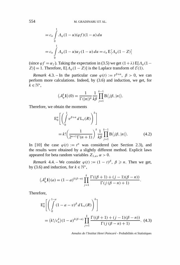
(ϕΛϕ)(1− u) (J−nαf )(1− u)duVol. 35, n◦ 4-1999.
554 M. GRADINARU ET AL.
= cn1∫
0
Λϕ(1− u)(ϕf )(1− u)du
= cn1∫
0
Λϕ(1− u)αf (1− u)du= cnE[Λϕ(1−Z)]
(sinceϕf = αf ). Taking the expectation in (3.5) we get(1+λ)E[Λϕ(1−Z)] = 1. Therefore, E[Λϕ(1−Z)] is the Laplace transform ofE(1).
Remark4.3. – In the particular caseϕ(t) := tβ+n, β > 0, we canperform more calculations. Indeed, by (3.6) and induction, we get, fork ∈N∗,
(Akϕ1
)(0)= 1
0(|n|)k1
kβ
k−1∏j=1
B(jβ, |n|).
Therefore, we obtain the moments
En0
[( 1∫0
vβ+n d Lv(R)
)k]
= k!(
1
2n+10(n+ 1)
)k 1
kβ
k−1∏j=1
B(jβ, |n|). (4.2)
In [10] the caseϕ(t) := tn was considered (see Section 2.3), andthe results were obtained by a slightly different method. Explicit lawsappeared for beta random variablesZ1,α, α > 0.
Remark4.4. – We considerϕ(t) := (1− t)β , β > n. Then we get,by (3.6) and induction, fork ∈N∗,
(Akϕ1
)(a)= (1− a)k(β−n)
k∏j=1
0((β + 1)+ (j − 1)(β − n))0(j (β − n)+ 1)
.
Therefore,
En0
[( 1−a∫0
(1− a − v)β d Lv(R)
)k]
= (k!/ckn)(1− a)k(β−n) k∏j=1
0((β + 1)+ (j − 1)(β − n))0(j (β − n)+ 1)
. (4.3)
Annales de l’Institut Henri Poincaré- Probabilités et Statistiques
ABEL TRANSFORM AND LOCAL TIMES 555
Remark4.5. – If we take in (3.7′) ϕ = 1 and a = 0, by the abovecalculations withβ = 0, we obtain the moment expressions
En0[(cn L1(R))
k]= k!/0(k|n| + 1), k ∈N∗, (4.4)
that is the moments of a Mittag-Leffler random variable with parame-ter |n| (see, e.g., [7], p. 447, or [14], p. 129; see also [5], p. 452). Thisis equivalent to the well known fact that the subordinator{τt : t > 0} isstable with index|n|:
En0[e−λτ1
]= e−cnλ|n|. (4.5)
Hereτ is the inverse of L(R), τt := inf{s: Ls(R) > t}, and satisfies thescaling property:
{τt : t > 0} (law)= {a τant : t > 0}.We can write, for anyk ∈N∗,
En0[(cn L1(R))
k]= En0
[cn/τ
k|n|1
]= ckn0(k|n|)−1
∞∫0
λk|n|−1 En0[e−λτ1
]dλ.
By (4.4),
∞∫0
λk|n|−1 En0[e−λτ1
]dλ= (k− 1)!/(|n|ckn)=
∞∫0
λk|n|−1 e−cnλ|n|dλ,
and we deduce (4.5), using the injectivity of the Mellin transform.Assuming (4.5), the above equality gives (4.4).
Proof of Corollary 3.4. –We simply take in (4.3),β = n to obtain thek-moments and the Laplace transform of(0(|n|)/2n+1)E(1). Then, byscaling, we note thatΛϕ does not depend ona ∈ [0,1[. The independenceproperty announced in the corollary also follows by scaling.2
Another proof of Corollary 3.4. –To prove (3.8), we may assume thatZ = 1, by scaling.(i) We denoteg := g1= sup{s 6 t : Rs = 0}. It is sufficient to prove that
At := 2n+10(|n|)−1
t∫0
(1− v)n d Lv(R), t ∈ [0,1], (a)
Vol. 35, n◦ 4-1999.
556 M. GRADINARU ET AL.
is the dual predictable projection ofCt := 1I{g6t}, t ∈ [0,1], that is
E[hg] = E
[ 1∫0
hv dAv
], (b)
for every predictable processh > 0 (see, e.g., [21], pp. 16–18). Indeed,we can follow the method in [2], p. 99. SinceAg = A1, taking in (b)h= exp(−λA), we have, for everyλ> 0,
E[exp(−λA1)
]=E
[ 1∫0
exp(−λAv) dAv]= E
[(1/λ)(1− exp(−λA1))
].
Thus, we obtain E[exp(−λA1)] = 1/(1+ λ), the desired result.(ii) We shall verify (b). It is enough to show this formula, forhv :=1I[0,T ](v), whereT is a stopping time with values in[0,1]:
P(g 6 T )= E[AT ]. (c)
Using (1.7), we can write
Px(T0> v)= 2n0(|n|)−1Φ(x2/v),
where we denotedΦ(y) := ∫ y0 s−n−1 e−s/2ds. Then,
P(g 6 T |FT )= 2n0(|n|)−1Φ(R2T /(1− T )
)= 2n0(|n|)−1Φ
(XT /(1− T ))
= 2n0(|n|)−1Ψ(R
2|n|T /(1− T )|n|).
Here we denotedΨ (y) := Φ(y1/|n|) and by{Xt : 06 t 6 1}, the squareof the Bessel process of indexn, whose infinitesimal generator is:
L= 2x(∂2/∂x2)+ 2(1+ n)(∂/∂x).
Clearly, (L + (∂/∂s))Φ(x/(1 − s)) = 0. Using the fact thatX|n|t −2|n|Lt (R) is a martingale (see Section 1.3), by Ito’s formula we can write
E[2n0(|n|)−1Φ
(XT /(1− T ))]
= E
[2n0(|n|)−1
T∫0
2|n|Ψ ′(0)(1− v)n d Lv(R)
].
Annales de l’Institut Henri Poincaré- Probabilités et Statistiques
ABEL TRANSFORM AND LOCAL TIMES 557
SinceΨ ′(0)= 1/|n|, we get
P(g 6 T )= 2n+10(|n|)−1 E
[ T∫0
(1− v)n d Lv(R)
]=E[AT ],
by (a), and (c) is verified. 2Remark4.6. – We can prove the following result which is, in some
sense, a reciprocal result of Corollary 3.4:Assume that, for anya ∈ [0,1[, the integral
1−a∫0
ϕ(a + v) d Lv(R) (3.8′)
is a standard exponential variable. Then
ϕ(t)= (2n+1/0(|n|))(1− t)n. (3.8′′)
For the proof, we note, by (3.4), that, for anya ∈ [0,1[, Λϕ(a) =1/(1+ λ). By Proposition 3.3,Λϕ verifies (3.5). HenceJ−n(ϕ)(a)= cn.Since, by (1.15),J−nεn = 0(n+ 1), we conclude using the injectivity ofAbel’s transform.
Proof of Proposition 3.5. –The right hand side of (3.1) can be writtenas (
2n+1/0(|n|))y 1∫0
sn−1 e−y2/2sf (1− s) ds
= (2n+1/0(|n|))y2n+1
1/y2∫0
un−1 e−1/2uf(1− uy2)du.
We replace in (3.1) (withλϕ instead ofϕ) the above equality, theexpression (1.1′) for pns (0, y) and we simplify byy2n+1. Then, lettingy ↓ 0, we get
2−n0(n+ 1)−1
1∫0
αf (1− s)s−n−1
×En0
[exp
(−λ
s∫0
ϕ(1− s + v) d Lv(r)
)]ds
Vol. 35, n◦ 4-1999.
558 M. GRADINARU ET AL.
= (1+ λ)−1(2n+1/0(|n|))f (1) ∞∫0
un−1 e−1/2u du
(recall thatϕf = αf ). Since (recall thatf (1)= 1/2)
(2n+1/0(|n|))f (1) ∞∫
0
un−1 e−1/2u du= 2f (1)= 1,
we get (3.10). To justify (3.9), we use (1.14′) and (2.12′):
1= 2(J−n(J n+1f ′)
)(1)= 2
(0(|n|))−1
1∫0
(1− s)−n−1(J n+1f ′)(s) ds
= 2−n0(n+ 1)−1
1∫0
s−n−1αf (1− s) ds. 2
Proof of Corollary 3.6. –The result is obtained takingf (t) =12tα−n−1 in Proposition 3.5. 2Proof of Proposition 3.7. –Let us denote
Λϕ(a;y) := En0
[exp
(−λ
1−a∫0
ϕ(a + v) d Lv(R)
)∣∣∣R1−a = y]
(a)
and
l(s) := (1− s)−n−1 e−y2/2(1−s)Λϕ(s;y). (b)
Clearly, Ξϕ(a) = Λϕ(a;0) and, for y = 0, l = ε−n−1 Ξϕ . With thesenotations and using (1.1′), (3.1), with λϕ instead ofϕ, can be writtenas
2−n0(n+ 1)−1
1∫0
(αf + λϕf )(s)l(s) ds
= (2n+1/0(|n|))y−2n
1∫0
sn−1 e−y2/2sf (1− s) ds. (c)
Taking in (c)f := δa , the Dirac delta function, and using (4.1), we obtain
Annales de l’Institut Henri Poincaré- Probabilités et Statistiques
ABEL TRANSFORM AND LOCAL TIMES 559
2n0(n+ 1)−1(1− a)nl(1)+ 2n(J n+1l′
)(1− a)
+ (λ0(|n|)/20(n+ 1))(ϕl)(a)
= 4ny−2n(1− a)n−1 e−y2/2(1−a).
Since, by (b),l(1)= 0, we get
2n(J n+1l′
)(a)+ (λ0(|n|)/(20(n+ 1))
)(ϕl)(a)
= 4ny−2nan−1 e−y2/2a,
or, by composition withJ−n,
l(a)+ (λ/cn) J−n(ϕε−n−1Λϕ(•;y))(a)= 2n0(−n)−1y−2n
a∫0
(a − u)−n−1un−1 e−y2/2u du. (d)
On the right hand side of (d), we make the change of variableu= vy2 toget
l(a)+ (λ/cn) J−n(ϕε−n−1Λϕ(•;y))(a)= 2n0(−n)−1
a/y2∫0
(a − vy2)−n−1
vn−1 e−1/2v dv.
Then, lettingy ↓ 0 in the above equality, we obtain,
a−n−1Ξϕ(a)+ (λ/cn)J−n(ϕε−n−1Ξϕ)(a)= a−n−1,
and making a straightforward calculation on its right hand side, weget (3.12). 2
Remark4.7. – By (3.14) we get the following moment expressions:for a ∈ [0,1], andk ∈N∗,
En0
[( 1−a∫0
ϕ(a + v) d Lv(r)
)k]= (k!/ckn)(Bkϕ1)(a). (3.14′)
Remark4.8. – We takeϕ(t) := tβ+n, β > 0. Then we get, by (3.6) andinduction, fork ∈N∗,
(Bkϕ1
)(0)= 1
0(|n|)kk∏j=1
B(jβ, |n|).
Vol. 35, n◦ 4-1999.
560 M. GRADINARU ET AL.
Therefore, we obtain the moments
En0
[( 1∫0
vβ+n d Lv(r)
)k]= k!
(1
2n+10(n+ 1)
)k k∏j=1
B(jβ, |n|). (4.6)
Remark4.9. – As in [10], Section 1.4, we can use the moment (orthe Laplace transform) formulas to deduce some limit theorems. Forexample, by (4.6) we can prove that, forβ ↓ 0,
2n+10(n+ 1)√δn
(√β
1∫0
vβ+n d Lv(r)− 1
2n+10(n+ 1)√β
)(law)−→N (0,1). (4.7)
Here,N (0,1) denotes the standard normal distribution and
δn := (0′(1)/0(1))− (0′(|n|)/0(|n|)),xB(x, |n|)= 1+ δnx + o(x), x ↓ 0.
The proof of this result is similar to the proof of Theorem 1.27 in [10].The same result can be obtained for the Bessel local time using (4.2): forβ ↓ 0,
2n+10(n+ 1)√δn
(√β
1∫0
vβ+n d Lv(R)− 1
2n+10(n+ 1)√β
)(law)−→N (0,1). (4.7′)
Remark4.10. – Proposition 3.5 can be obtained as a consequence ofProposition 3.7. ConsiderZ a random variable with density
2−n0(n+ 1)−1s−n−1αf (1− s)1I[0,1](s),independent from the Bessel bridger. We compute
E[(BϕΞϕ)(1−Z)]= E
[Zn+1J−n
(ϕε−n−1Ξϕ
)(Z)
]= 2−n0(n+ 1)−10(−n)
1∫0
αf (1− s) ds
×s∫
0
(s − u)−n−1(ϕΞϕ)(u)u−n−1 du
Annales de l’Institut Henri Poincaré- Probabilités et Statistiques
ABEL TRANSFORM AND LOCAL TIMES 561
= 2−n0(n+ 1)−10(−n)1∫
0
(ϕΞϕ
)(u)u−n−1 du
×1−u∫0
(1− u− v)−n−1αf (v) dv
= 2−n0(n+ 1)−1
1∫0
(ϕ Ξϕ)(1− u)u−n−1(J−nαf )(1− u)du= 20(|n|)−1
1∫0
Ξϕ(1− u)u−n−1(ϕf )(1− u)du
= 20(|n|)−1
1∫0
Ξϕ(1− u)u−n−1αf (1− u)du= cnE[Ξϕ(1−Z)](since αf = ϕf ). Then, we take the expectation in (3.12) and wededuce (3.10).
Remark4.11. – We can obtain (3.3) from (3.10) and vice-versa.Indeed, by (1.10), it is not difficult to see that
(Lt (r)
)t∈[0,1]
(law)= (gn Lg t (R)
)t∈[0,1]. (4.8)
Here, we denoteg := g1 = sup{s < 1: Rs = 0} which is independentfrom (g−1/2Rg t : t 6 1), hence from(gn Lg t (R): t > 0). From (4.8), weobtain that, for any positive Borel functionψ ,
g|n|1∫
0
ψ(gv) d Lv(r)(law)=
1∫0
ψ(v) d Lv(R).
Recall that (see Section 1.4)g is a beta random variable with parameters−n,n+ 1. Then, by (3.14), to deduce (3.7) (both fora = 0), we need toverify, for anyk ∈N∗,(Akϕ1
)(0)= B(−n,n+ 1)−1
1∫0
t−n−1(1− t)nt−kn(Bkϕ(t •)1)(0) dt. (4.9)
Fork = 1 we can write, by (3.13),
Vol. 35, n◦ 4-1999.
562 M. GRADINARU ET AL.
B(−n,n+ 1)−1
1∫0
t−n−1(1− t)nt−kn(Bkϕ(t •)1)(0) dt= B(−n,n+ 1)−10(−n)−1
1∫0
t−n−1(1− t)nt−n dt
×1∫
0
(1− u)−n−1ϕ(t (1− u))u−n−1 du
= B(−n,n+1)−10(−n)−1
1∫0
v−n−1ϕ(v) dv
1∫v
(1− t)n(t−v)−n−1dt
= 0(−n)−1
1∫0
v−n−1ϕ(v) dv = (Aϕ1)(0),
as we can see by making the changes of variablest (1− u) = v ands = (t −v)/(1−v). The same reasoning applies for arbitraryk. We leaveto the reader the proof of the fact that (3.14) can be obtained by (3.7).
Remark4.12. – Assume that the conditioning is{R1−a = y}, witharbitraryy. Then a functional equation, similar to (3.5), can be written,using (3.1): (
I + (λ/cn)Aϕ)Ψϕ(•;y)=ψ(•;y), (4.10)
where
Ψϕ(a;y) :=pn1−a(0, y)
×En0
[exp
(−λ
1−a∫0
ϕ(a + v) d Lv(R)
)∣∣∣R1−a = y]
(4.11)
and
ψ(a;y) := 0(n+ 1)−10(−n)−1y
a∫0
(a − u)−n−1un−1 e−y2/2u du. (4.12)
Therefore, we get a similar expression as (3.7) forΨϕ(a;y) with ψ(•;y)instead of the constant function1.
Annales de l’Institut Henri Poincaré- Probabilités et Statistiques
ABEL TRANSFORM AND LOCAL TIMES 563
Remark4.13. – Here, we give a probabilistic explanation for theappearance of Abel’s integral operator, using the Bessel meander. In fact,we can state a reciprocal result of Theorem 3.1:
Consider the continuous functionf : [0,1] → [0,∞[, such thatf ∈C1(]0,1]), f (0) = 0, and assume that the random variableZ isindependent from the Bessel processR, having the probability densityfunctionβ(1− s)1I[0,1](s). Suppose that the random variableRZ has theprobability density function given by
k−1f
(2n+1/0(|n|))y1I[0,∞[(y)
1∫0
sn−1 e−y2/2sf (1− s) ds. (4.13)
Then, the functionβ is an Abel transform off ′. More precisely,
β(t)= αf (t)= cn(J n+1f ′)(t). (4.14)
For the proof, we recall that, by (1.12) and (1.12′),
Rt(law)= √t − gt mt(1),
andmt(1) is independent ofgt , being Rayleigh distributed. Let us denote,for any positive bounded Borel functionh,
Φh(s) :=∞∫
0
h(y√s)y e−y
2/2dy.
Then, by (4.13),
1∫0
β(s)En0[Φh(s − gs)]ds = k−1
f
(2n+1/0(|n|)) 1∫
0
snΦh(s)f (s) ds.
Hence, the probability density function of the random variableZ− gZ is
k−1f
(2n+1/0(|n|))snf (s)1I[0,1](s). (a)
On the other hand,Z − gZ (law)= Z(1− g1), with g1 independent fromZ.Recall that 1− g1 is a beta random variable with parametersn+ 1,−n.Hence,
Vol. 35, n◦ 4-1999.
564 M. GRADINARU ET AL.
E[l(Z− gZ)]= B(n+ 1,−n)−1
1∫0
l(y) dy
1∫y
un(1− u)−n−1β(y/u) du, (b)
for any positive bounded Borel functionl on[0,1]. Combining (a) and (b)we get, fory ∈ [0,1],k−1f
(2n+1/0(|n|))(1− y)nf (y)= 0(n+ 1)−10(−n)−1
1∫1−y
un(1− u)−n−1β(1− (1− y)/u) du. (c)
We make on the right hand side of (c) the change of variablev =1− (1− y)/u and we get, after straightforward calculations,
f (y)= (1/cn)(J−nβ)(y).We get the same result by composition withJ−n in (4.14).
APPENDIX A. FORMULAE ON INTEGRALS OF BESSELLOCAL TIMES
We gather here the main results obtained in [10] (these are denotedbetween brackets) and in the present paper.
Explicit laws
We denote by Lt (B) and Lt (b) the local times at 0 of the Brownianmotion B starting from 0, and of the Brownian bridgeb; we denoteby Lt (R) and Lt (r) the local times at 0 of the Bessel processR, ofindexn∈]−1,0[, starting from 0, and of the Bessel bridger. Here,Za,bdenotes a beta random variable with parametersa, b independent of theprocess for which the local time is considered; in particularU = Z1,1 isa uniform random variable on[0,1] andV = Z 1
2 ,12
is an arcsine randomvariable.E(1) is the standard exponential distribution andγ (2) is thegamma distribution of parameter 2.c denotes a normalisation constant.The last passage time in 0 before time 1 is denotedg = sup{s 6 1: Bsor Rs = 0}. Z is independent of the process for which the local timeis considered.λ is a strictly positive parameter. Iff ∈ C1(R∗+), with
Annales de l’Institut Henri Poincaré- Probabilités et Statistiques
ABEL TRANSFORM AND LOCAL TIMES 565
f (0)= 0, we denote byαf the function
αf (t)= (2n+1/0(|n|)) t∫0
(t − u)nf ′(u) du.
(1) Brownian motion
√2π
B(12, λ)
Z1,λ∫0
d Lt (B)√1−Z1,λ + t
(law)= E(1) [1.18] (B1)
√2π
B(λ, 12)
1∫0
d Lt (B)√t + Zλ,1
1−Zλ,1
(law)=√π
2
1∫0
d Lt (B)√t + U
1−U
(law)= E(1)
[1.25,1.26] (B2)
√2π
B(λ, 12)
√1−Zλ, 1
2
∞∫0
d Lt (B)√(1+ t) (t +Zλ, 1
2)
(law)= E(1) [2.25] (B3)
√2
π
1∫0
d Lt (B)√1− t
(law)=√
2
π
∞∫1
d Lt (B)√t (t − 1)
(law)= E(1)
[1.23,A.16], see also [A] (B4)
a
∞∫0
d Lat (B)
t
(law)= E(1),
(La local time at levela) [Rk.1.26, iv)] (B5)√
2L1(B)(law)= √2|B1| (law)= Mittag-Leffler
(12
)[Rk.1.26, i)], (4.4) (B6)
(2) Brownian bridge
√2π
B(λ, 12)
1∫0
d Lt (b)√t +
Zλ, 12
1−Zλ, 12
(law)= E(1) [1.31] (b1)
Vol. 35, n◦ 4-1999.
566 M. GRADINARU ET AL.√2
π
1∫0
d Lt (b)√t + V
1−V
(law)=√
2
π
1∫0
d Lt (b)√1V− t
(law)= E(1) [1.32] (b2)
√2
π
1∫0
d Lt (b)√t + 1−g
g
(law)= E(1) (g(law)= Z 1
2 ,12
) [1.34] (b3)
√2
π
1∫0
d Lt (b)√t + Z
1−Z
(law)= γ (2),
Z(law)= 1
cπ
log 1/u√u(1− u)1I[0,1](u) [1.36] (b4)
1√π
12∫
0
d Lt (b)√(1
2 − t)(1− t)(law)= 1√
π
1∫12
d Lt (b)√t (t − 1
2)
(law)= E(1)
[1.23,A.16] (b5)
L1(b)(law)= √
2E(1) [Rk.1.26, iv)] (b6)
(3) Bessel process
2|n|Z∫
0
ϕ(1−Z+ t) d Lt (R)(law)= E(1),
Z(law)= cαf (1− u)1I[0,1](u) (3.3) (R1)
2n+10(n+ 1)
B(|n|, λ)Z1,λ∫0
(1−Z1,λ + t)n d Lt (R)(law)= E(1) [2.37], (3.3) (R2)
2n+10(n+ 1)
B(|n|, λ)
Z1,λ1−Z1,λ∫0
(1+ t)n d Lt (R)(law)= E(1) [2.37], (3.3) (R3)
2n+1
0(|n|)Z1,n+1∫
0
(1−Z1,n+1+ t)n d Lt (R)(law)= E(1) [2.37], (3.3) (R4)
Annales de l’Institut Henri Poincaré- Probabilités et Statistiques
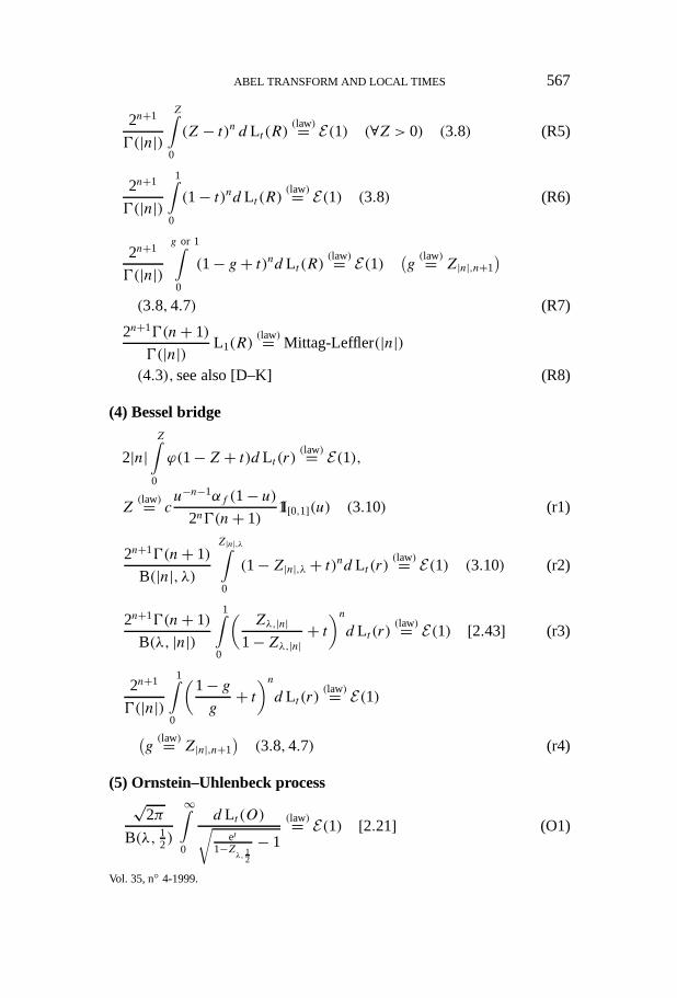
ABEL TRANSFORM AND LOCAL TIMES 567
2n+1
0(|n|)Z∫
0
(Z − t)n d Lt (R)(law)= E(1) (∀Z > 0) (3.8) (R5)
2n+1
0(|n|)1∫
0
(1− t)nd Lt (R)(law)= E(1) (3.8) (R6)
2n+1
0(|n|)g or 1∫0
(1− g+ t)nd Lt (R)(law)= E(1) (
g(law)= Z|n|,n+1
)(3.8,4.7) (R7)
2n+10(n+ 1)
0(|n|) L1(R)(law)= Mittag-Leffler(|n|)
(4.3),see also [D–K] (R8)
(4) Bessel bridge
2|n|Z∫
0
ϕ(1−Z+ t)d Lt (r)(law)= E(1),
Z(law)= c
u−n−1αf (1− u)2n0(n+ 1)
1I[0,1](u) (3.10) (r1)
2n+10(n+ 1)
B(|n|, λ)Z|n|,λ∫0
(1−Z|n|,λ + t)nd Lt (r)(law)= E(1) (3.10) (r2)
2n+10(n+ 1)
B(λ, |n|)1∫
0
(Zλ,|n|
1−Zλ,|n| + t)nd Lt (r)
(law)= E(1) [2.43] (r3)
2n+1
0(|n|)1∫
0
(1− gg+ t)nd Lt (r)
(law)= E(1)
(g(law)= Z|n|,n+1
)(3.8,4.7) (r4)
(5) Ornstein–Uhlenbeck process√
2π
B(λ, 12)
∞∫0
d Lt (O)√et
1−Zλ, 12
− 1
(law)= E(1) [2.21] (O1)
Vol. 35, n◦ 4-1999.
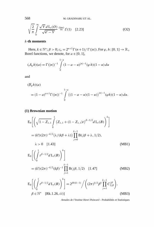
568 M. GRADINARU ET AL.√2
π
∞∫0
√V d Lt (O)√
et − V(law)= E(1) [2.23] (O2)
k-th moments
Here,k ∈N∗; β > 0; cn = 2n+10(n+1)/0(|n|). Forϕ,h : [0,1]→R+Borel functions, we denote, fora ∈ [0,1],
(Aϕh)(a)= 0(|n|)−1
1−a∫0
(1− a − u)|n|−1(ϕ h)(1− u)du
and
(Bϕh)(a)
= (1− a)n+10(|n|)−1
1−a∫0
((1− a − u)(1− u))|n|−1
(ϕh)(1− u)du.
(1) Brownian motion
E0
[(√1−Zλ,1
1∫0
(Zλ,1+ (1−Zλ,1)t)β−1/2
d Lt (B)
)k]
= (k!)(2π)−k/2(λ/(kβ + λ)) k−1∏j=0
B(jβ + λ,1/2),
λ > 0 [1.43] (MB1)
E0
[( 1∫0
tβ−1/2d Lt (B)
)k]
= (k!)(2π)−k/2(kβ)−1k−1∏j=1
B(jβ,1/2) [1.47] (MB2)
E0
[( 1∫0
tβ−1/2d Lt (B)
)k]= 2βk(k−1)
/((2π)k/2βk
k−1∏j=1
Cjβ2jβ
),
β ∈N∗ [Rk.1.26, ii)] (MB3)
Annales de l’Institut Henri Poincaré- Probabilités et Statistiques
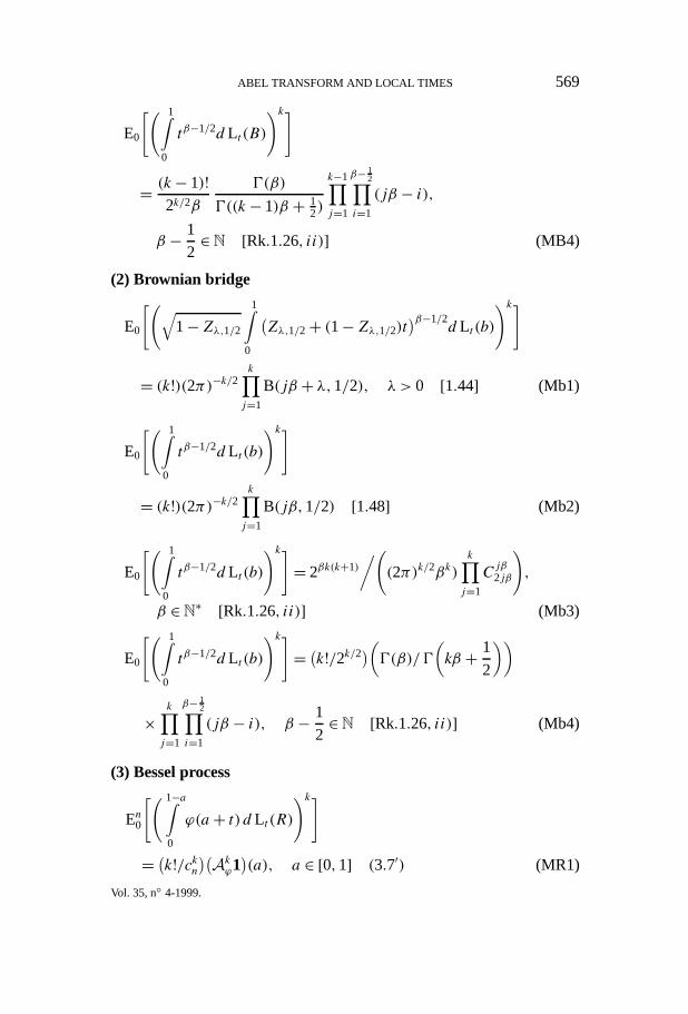
ABEL TRANSFORM AND LOCAL TIMES 569
E0
[( 1∫0
tβ−1/2d Lt (B)
)k]
= (k− 1)!2k/2β
0(β)
0((k− 1)β + 12)
k−1∏j=1
β− 12∏
i=1
(jβ − i),
β − 1
2∈N [Rk.1.26, ii)] (MB4)
(2) Brownian bridge
E0
[(√1−Zλ,1/2
1∫0
(Zλ,1/2+ (1−Zλ,1/2)t)β−1/2
d Lt (b)
)k]
= (k!)(2π)−k/2k∏j=1
B(jβ + λ,1/2), λ > 0 [1.44] (Mb1)
E0
[( 1∫0
tβ−1/2d Lt (b)
)k]
= (k!)(2π)−k/2k∏j=1
B(jβ,1/2) [1.48] (Mb2)
E0
[( 1∫0
tβ−1/2d Lt (b)
)k]= 2βk(k+1)
/((2π)k/2βk)
k∏j=1
Cjβ2jβ
),
β ∈N∗ [Rk.1.26, ii)] (Mb3)
E0
[( 1∫0
tβ−1/2d Lt (b)
)k]= (k!/2k/2)(0(β)/0(kβ + 1
2
))
×k∏j=1
β− 12∏
i=1
(jβ − i), β − 1
2∈N [Rk.1.26, ii)] (Mb4)
(3) Bessel process
En0
[( 1−a∫0
ϕ(a + t) d Lt (R)
)k]
= (k!/ckn)(Akϕ1)(a), a ∈ [0,1] (3.7′) (MR1)
Vol. 35, n◦ 4-1999.
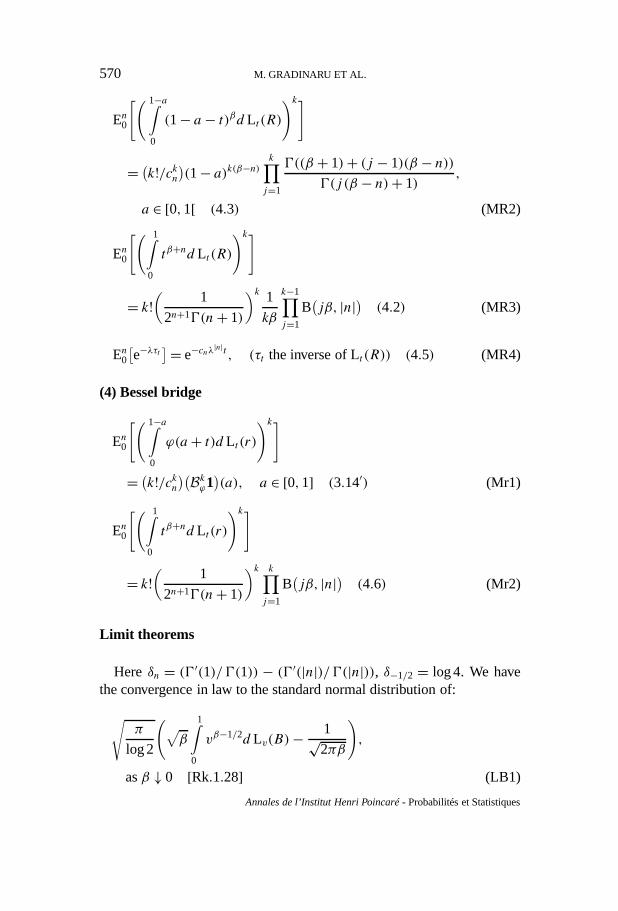
570 M. GRADINARU ET AL.
En0
[( 1−a∫0
(1− a − t)βd Lt (R)
)k]
= (k!/ckn)(1− a)k(β−n) k∏j=1
0((β + 1)+ (j − 1)(β − n))0(j (β − n)+ 1)
,
a ∈ [0,1[ (4.3) (MR2)
En0
[( 1∫0
tβ+nd Lt (R)
)k]
= k!(
1
2n+10(n+ 1)
)k 1
kβ
k−1∏j=1
B(jβ, |n|) (4.2) (MR3)
En0[e−λτt
]= e−cnλ|n|t , (τt the inverse of Lt (R)) (4.5) (MR4)
(4) Bessel bridge
En0
[( 1−a∫0
ϕ(a+ t)d Lt (r)
)k]
= (k!/ckn)(Bkϕ1)(a), a ∈ [0,1] (3.14′) (Mr1)
En0
[( 1∫0
tβ+nd Lt (r)
)k]
= k!(
1
2n+10(n+ 1)
)k k∏j=1
B(jβ, |n|) (4.6) (Mr2)
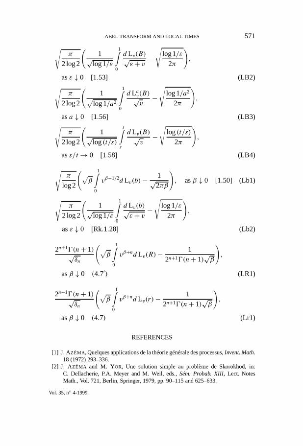
Limit theorems
Here δn = (0′(1)/0(1)) − (0′(|n|)/0(|n|)), δ−1/2 = log 4. We havethe convergence in law to the standard normal distribution of:
√π
log 2
(√β
1∫0
vβ−1/2d Lv(B)− 1√2πβ
),
asβ ↓ 0 [Rk.1.28] (LB1)
Annales de l’Institut Henri Poincaré- Probabilités et Statistiques
ABEL TRANSFORM AND LOCAL TIMES 571√π
2 log 2
(1√
log1/ε
1∫0
d Lv(B)√ε+ v −
√log1/ε
2π
),
asε ↓ 0 [1.53] (LB2)√π
2 log 2
(1√
log 1/a2
1∫0
d Lav(B)√v−√
log 1/a2
2π
),
asa ↓ 0 [1.56] (LB3)√π
2 log 2
(1√
log(t/s)
t∫s
d Lv(B)√v−√
log(t/s)
2π
),
ass/t→ 0 [1.58] (LB4)
√π
log 2
(√β
1∫0
vβ−1/2d Lv(b)− 1√2πβ
), asβ ↓ 0 [1.50] (Lb1)
√π
2 log 2
(1√
log 1/ε
1∫0
d Lv(b)√ε+ v −
√log 1/ε
2π
),
asε ↓ 0 [Rk.1.28] (Lb2)
2n+10(n+ 1)√δn
(√β
1∫0
vβ+nd Lv(R)− 1
2n+10(n+ 1)√β
),
asβ ↓ 0 (4.7′) (LR1)
2n+10(n+ 1)√δn
(√β
1∫0
vβ+nd Lv(r)− 1
2n+10(n+ 1)√β
),
asβ ↓ 0 (4.7) (Lr1)
REFERENCES
[1] J. AZÉMA, Quelques applications de la théorie générale des processus,Invent. Math.18 (1972) 293–336.
[2] J. AZÉMA and M. YOR, Une solution simple au problème de Skorokhod, in:C. Dellacherie, P.A. Meyer and M. Weil, eds.,Sém. Probab. XIII, Lect. NotesMath., Vol. 721, Berlin, Springer, 1979, pp. 90–115 and 625–633.
Vol. 35, n◦ 4-1999.
572 M. GRADINARU ET AL.
[3] M. BAXTER and D. WILLIAMS , Symmetry characterizations of certain distribu-tions 1,Math. Proc. Camb. Phil. Soc.111 (1992) 387–399.
[4] M. BAXTER and D. WILLIAMS , Symmetry characterizations of certain distribu-tions 2,Math. Proc. Camb. Phil. Soc.112 (1992) 599–611.
[5] J. BERTOIN and M. YOR, Some independence results related to the arcsine law,J. Theor. Probab.9 (1996) 447–458.
[6] A.N. BORODIN and P. SALMINEN , Handbook of Brownian Motion: Facts andFormulae, Birlehäuser, Berlin, 1996.
[7] D.A. DARLING and M. KAC, On occupation times for Markov processes,Trans.Amer. Math. Soc.84 (1957) 444–458.
[8] R.K. GETOOR, The Brownian escape process,Ann. Probab.7 (1979) 864–867.[9] R. GORENFLOand S. VESSELLA, Abel Integral Equations: Analysis and Applica-
tions, Lect. Notes Math., Vol. 1461, Springer, Berlin, 1991.[10] M. GRADINARU, B. ROYNETTE, P. VALLOIS and M. YOR, The laws of Brownian
local time integrals, Prépublication No. 38-1997, Institut Élie Cartan, UniversitéHenri Poincaré (Vandœuvre-lès-Nancy, France); to appear inComputational andApplied Mathematics, Birkhäuser, Boston, 1999.
[11] K. I TO and H.P. MCKEAN, Diffusion Processes and Their Sample Paths, Springer,Berlin, 1965.
[12] TH. JEULIN, Semi-martingales et Grossissement d’une Filtration, Lect. NotesMath., Vol. 833, Springer, Berlin, 1980.
[13] J. KENT, Some probabilistic properties of Bessel functions,Ann. Probab.6 (1978)760–770.
[14] S.A. MOLCHANOV and E. OSTROVSKII, Symmetric stable processes as traces ofdegenerate diffusion processes,Theoty Probab. Appl.14 (1969) 128–131.
[15] J.W. PITMAN and M. YOR, Bessel processes and infinitely divisible laws, in:D. Williams, ed.,Stochastic Integrals, Lect. Notes Math., Vol. 851, Springer,Berlin, 1981, pp. 285–370.
[16] B. RAJEEV and M. YOR, Local times and almost sure convergence of semi-martingales,Ann. Inst. Henri Poincaré31 (1995) 653–667.
[17] D. REVUZ and M. YOR, Continuous Martingales and Brownian Motion, 2nd Ed.,Springer, Berlin, 1994.
[18] M.J. SHARPE, Some transformations of diffusions by time reversal,Ann. Probab.8(1980) 1157–1162.
[19] S. SATO and M. YOR, Computations of moments for discounted Brownian additivefunctionals,J. Math. Kyoto38 (3) (1998) 475–486.
[20] M. YOR, Some Aspects of Brownian Motion I: Some Special Functionals,Birkhäuser, Basel, 1992.
[21] M. YOR, Local Times and Excursions for Brownian Motion: A Concise Introduc-tion, Caracas-Paris, 1996.
[22] M. YOR, Some Aspects of Brownian Motion II: Some Recent Martingale Problems,Birkhäuser, Berlin, 1997.
[23] M. YOR, On certain discounted arcsine laws,Stochastic Process. Appl.71 (1997)111–122.
Annales de l’Institut Henri Poincaré- Probabilités et Statistiques


![02 ter- Transform es de Laplace [Mode de compatibilit ]](https://img.pdfslide.fr/doc/110x75/62bb6809eafa5e2c3f317ff0/02-ter-transform-es-de-laplace-mode-de-compatibilit-.jpg)