Analyse Experiment Ale Cours

8/9/2019 Analyse Experiment Ale Cours

http://slidepdf.com/reader/full/analyse-experiment-ale-cours 1/12

+UC-SDRL-RJA CN-20-263-663/664 Revision: June 7, 1999 +

1. EXPERIMENTAL MODAL ANALYSIS

1.1 Introduction

Experimental modal analysis is the process of determining the modal parameters (frequencies,

damping factors, modal vectors and modal scaling) of a linear, time invariant system by way of

an experimental approach. The modal parameters may be determined by analytical means, such

as finite element analysis, and one of the common reasons for experimental modal analysis is the

verification/correction of the results of the analytical approach (model updating). Often, though,

an analytical model does not exist and the modal parameters determined experimentally serve as

the model for future evaluations such as structural modifications. Predominately, experimental

modal analysis is used to explain a dynamics problem, vibration or acoustic, that is not obvious

from intuition, analytical models, or previous similar experience. It is important to remember

that most vibration and/or acoustic problems are a function of both the forcing functions (or

initial conditions) and the system characteristics described by the modal parameters. Modal

analysis alone is not the answer to the whole problem but is often an important part of the

process. Likewise, many vibration and/or acoustic problems fall outside of the assumptions

associated with modal analysis (linear superposition, for example). For these situations, modal

analysis may not be the right approach and an analysis that focuses on the specific characteristics

of the problem will be more useful.

The history of experimental modal analysis began in the 1940’s with work oriented toward

measuring the modal parameters of aircraft so that the problem of flutter could be accurately

predicted. At that time, transducers to measure dynamic force were primitive and the analog

nature of the approach yielded a time consuming process that was not practical for most

situations. With the advent of digital mini-computers and the Fast Fourier Transform (FFT) in

the 1960’s, the modern era of experimental modal analysis began. Today, experimental modal

analysis represents an interdisciplinary field that brings together the signal conditioning and

computer interaction of electrical engineering, the theory of mechanics, vibrations, acoustics, and

control theory from mechanical engineering, and the parameter estimation approaches of applied

mathematics[1-12]

.

(1-1)




1.2 Experimental Modal Analysis Overview

The process of determining modal parameters from experimental data involves several phases.

While these phases can be, in the simplest cases, very abbreviated, experimental modal analysis

depends upon the understanding of the basis for each phase. As in most experimental situations,

the success of the experimental modal analysis process depends upon having very specific goals

for the test situation. Such specific goals affect every phase of the process in terms of reducing

the errors associated with that phase. While there are several ways of breaking down the process,

one possible delineation of these phases is as follows:

• Modal Analysis Theory

• Experimental Modal Analysis Methods

• Modal Data Acquisition

• Modal Parameter Estimation

• Modal Data Presentation/Validation

Modal analysis theory refers to that portion of classical vibrations that explains, theoretically, the

existence of natural frequencies, damping factors, and mode shapes for linear systems. This

theory includes both lumped parameter, or discrete, models as well as continuous models. This

theory also includes real normal modes as well as complex modes of vibration as possible

solutions for the modal parameters. This phase of the experimental modal analysis process will

not be repeated here but is summarized in Analytical and Experimental Modal Analysis (UC-

SDRL-CN-20-263-662) as well as in other textbooks on vibration[1-4]

. The relationships of

transforms to vibration theory is very important to the comprehension of modern experimental

modal analysis methods. Particularly, since discrete Fourier transforms are often involved in the

modal data acquisition phase, this aspect of modal theory is critical.

Experimental modal analysis methods involve the theoretical relationship between measured

quantities and the classic vibration theory often represented as matrix differential equations. All

modern methods trace from the matrix differential equations but yield a final mathematical form

in terms of measured data. This measured data can be raw input and output data in the time or

frequency domains or some form of processed data such as impulse response or frequency

response functions. Most current methods involve processed data such as frequency response

(1-2)




functions in the estimation of modal parameters. In summary, though, the experimental modal

analysis method establishes the form of the data that must be acquired.

Modal data acquisition involves the practical aspects of acquiring the data that is required as

input to the modal parameter estimation phase. Therefore, a great deal of care must be taken to

assure that the data matches the requirements of the theory as well as the requirements of the

numerical algorithm involved in the modal parameter estimation. This phase involves both the

digital signal processing and measurement (frequency response function) formulation. The

theoretical requirements involve concerns such as system linearity as well as time invariance of

system parameters. It is very important, in this phase, to understand the origin of errors, both

variance and bias, in the measurement process. Certain bias errors, which originate due to

limitations of the fast Fourier transform (FFT) may seriously compromise the estimates of modal

parameters[5-8]

.

Modal parameter estimation is concerned with the practical problem of estimating the modal

parameters, based upon a choice of mathematical model as justified by the experimental modal

analysis method, from the measured data. Problems which occur at this phase most often arise

from violations of assumptions used in previous phases. Serious theoretical problems such as

nonlinear considerations cause serious problems in the estimation of modal parameters and may

be reason to completely invalidate the experimental modal analysis approach. Serious practical

problems such as bias errors resulting from the digital signal processing will cause similar

problems but are a function of data acquisition techniques which can be altered to minimize such

errors. The modal parameter estimation phase is that point in the experimental modal analysis

process where the errors of all previous work are accumulated[9-12]

.

Modal data presentation/validation is that process of providing a physical view or interpretation

of the modal parameters. For example, this may simply be the numerical tabulation of the

frequency, damping, and modal vectors along with the associated geometry of the measured

degrees of freedom. More often, modal data presentation involves the plotting and animation of such information. This involves the additional information required to construct a three

dimensional representation of the test object. Primarily, this requires a display sequence

involving the order in which the degrees of freedom will be connected. Newer approaches to the

plotting and animation of the modal vectors involve hidden line calculations which require

surface definition as well.

(1-3)




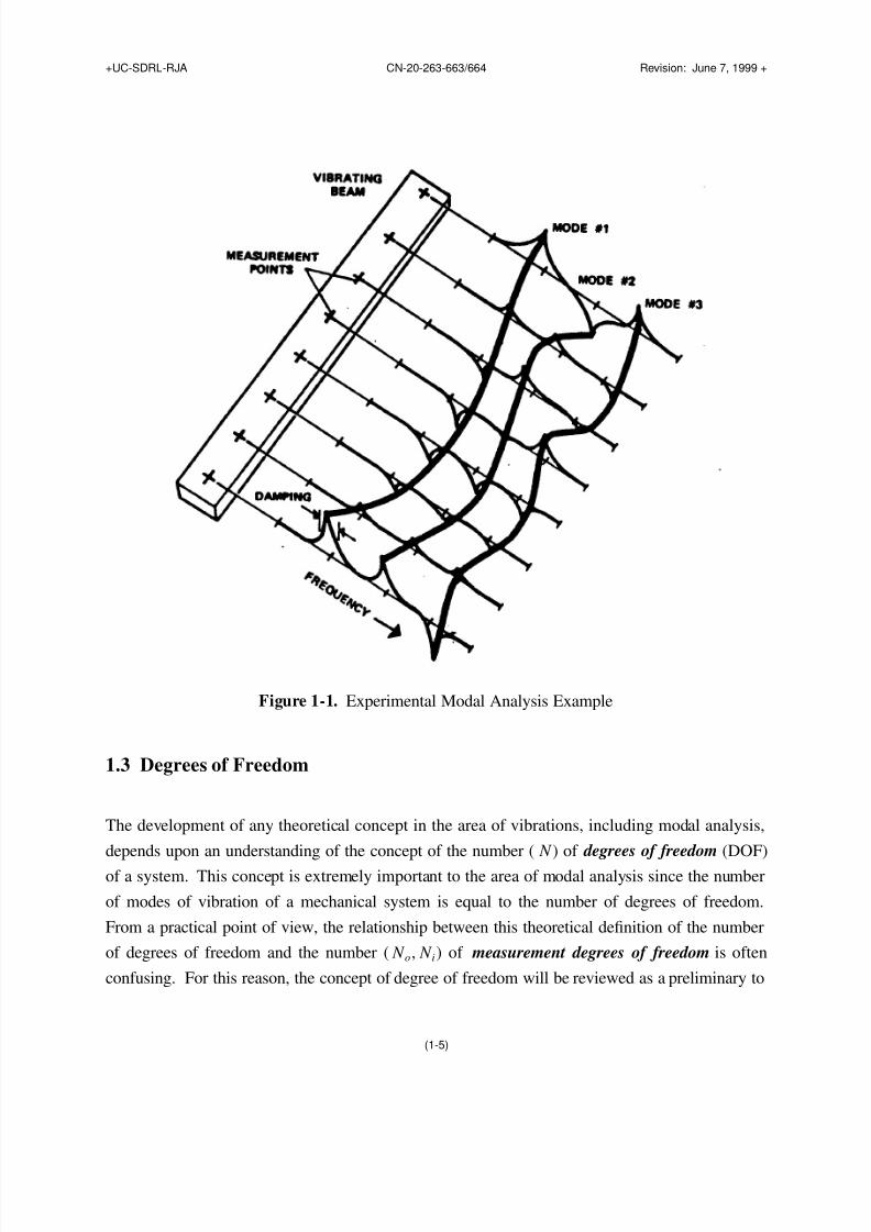
Figure 1-1 is a representation of all phases of the process. First of all, a continuous beam is

being evaluated for the first few modes of vibration. Modal analysis theory explains that this is a

linear system and that the modal vectors of this system should be real normal modes. The

experimental modal analysis method that has been used is based upon the frequency response

function relationships to the matrix differential equations of motion. At each measured degree of

freedom the imaginary part of the frequency response function for that measured response degree

of freedom and a common input degree of freedom is superimposed perpendicular to the beam.

Naturally, the modal data acquisition involved in this example involves the estimation of

frequency response functions for each degree of freedom shown. Note that the frequency

response functions are complex valued functions and that only the imaginary portion of each

function is shown. One method of modal parameter estimation suggests that for systems with

light damping and widely spaced modes, the imaginary part of the frequency response function,

at the damped natural frequency, may be used as an estimate of the modal coefficient for that

response degree of freedom. The damped natural frequency can be identified as the frequency of

the positive and negative peaks in the imaginary part of the frequency response functions. The

damping can be estimated from the sharpness of the peaks. In this very simple way, the modal

parameters have been estimated. Modal data presentation for this case is shown as the lines

connecting the peaks. While animation is possible, a reasonable interpretation of the modal

vector can be gained in this simple case from plotting alone.

(1-4)




Figure 1-1. Experimental Modal Analysis Example

1.3 Degrees of Freedom

The development of any theoretical concept in the area of vibrations, including modal analysis,

depends upon an understanding of the concept of the number ( N ) of degrees of freedom (DOF)

of a system. This concept is extremely important to the area of modal analysis since the number

of modes of vibration of a mechanical system is equal to the number of degrees of freedom.

From a practical point of view, the relationship between this theoretical definition of the number

of degrees of freedom and the number ( N o, N i) of measurement degrees of freedom is often

confusing. For this reason, the concept of degree of freedom will be reviewed as a preliminary to

(1-5)




the following experimental modal analysis material.

To begin with, the basic definition that is normally associated with the concept of the number of

degrees of freedom involves the following statement: The number of degrees of freedom for a

mechanical system is equal to the number of independent coordinates (or minimum number of

coordinates) that is required to locate and orient each mass in the mechanical system at any

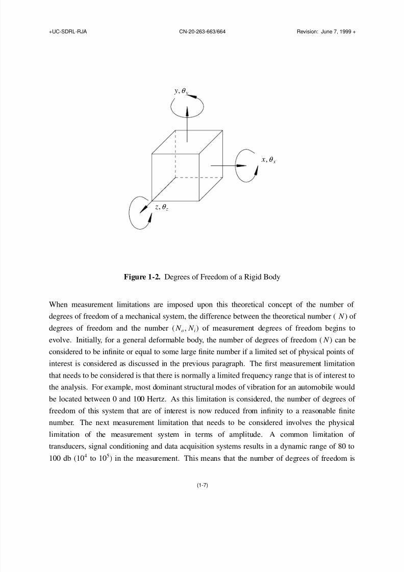
instant in time. As this definition is applied to a point mass, three degrees of freedom are

required since the location of the point mass involves knowing the x, y, and z translations of the

center of gravity of the point mass. As this definition is applied to a rigid body mass, six degrees

of freedom are required since θ x , θ y, and θ z rotations are required in addition to the x, y, and z

translations in order to define both the orientation and location of the rigid body mass at any

instant in time. This concept is represented in Figure 1-2. As this definition is extended to any

general deformable body, it should be obvious that the number of degrees of freedom can now be

considered as infinite. While this is theoretically true, it is quite common, particularly with

respect to finite element methods, to view the general deformable body in terms of a large

number of physical points of interest with six degrees of freedom for each of the physical points.

In this way, the infinite number of degrees of freedom can be reduced to a large but finite

number.

(1-6)




x,θ x

y,θ y

z,θ z

Figure 1-2. Degrees of Freedom of a Rigid Body

When measurement limitations are imposed upon this theoretical concept of the number of

degrees of freedom of a mechanical system, the difference between the theoretical number ( N ) of

degrees of freedom and the number ( N o, N i) of measurement degrees of freedom begins to

ev olve. Initially, for a general deformable body, the number of degrees of freedom ( N ) can be

considered to be infinite or equal to some large finite number if a limited set of physical points of

interest is considered as discussed in the previous paragraph. The first measurement limitation

that needs to be considered is that there is normally a limited frequency range that is of interest to

the analysis. For example, most dominant structural modes of vibration for an automobile would

be located between 0 and 100 Hertz. As this limitation is considered, the number of degrees of freedom of this system that are of interest is now reduced from infinity to a reasonable finite

number. The next measurement limitation that needs to be considered involves the physical

limitation of the measurement system in terms of amplitude. A common limitation of

transducers, signal conditioning and data acquisition systems results in a dynamic range of 80 to

100 db (104 to 105) in the measurement. This means that the number of degrees of freedom is

(1-7)




reduced further due to the dynamic range limitations of the measurement instrumentation.

Finally, since few rotational transducers exist at this time, the normal measurements that are

made involve only translational quantities (displacement, velocity, acceleration, force) and thus

do not include rotational degrees-of-freedom (RDOF). In summary, even for the general

deformable body, the theoretical number of degrees of freedom that are of interest are limited to

a very reasonable finite value ( N = 1 − 50). Therefore, this number of degrees of freedom ( N ) is

the number of modes of vibration that are of interest.

Finally, then, the number of measurement degrees of freedom ( N o, N i) can be defined as the

number of physical locations at which measurements are made times the number of

measurements made at each physical location. For example, if x, y, and z accelerations are

measured at each of 100 physical locations on a general deformable body, the number of

measurement degrees of freedom would be equal to 300. It should be obvious that since the

physical locations are chosen somewhat arbitrarily, and certainly without exact knowledge of the

modes of vibration that are of interest, that there is no specific relationship between the number

of degrees of freedom ( N ) and the number of measurement degrees of freedom ( N o, N i). In

general, in order to define N modes of vibration of a mechanical system, N o, N i must be equal to

or larger than N . Even though N o, N i is larger than N , this is not a guarantee that N modes of

vibration can be found from N o, N i measurement degrees of freedom. The N o, N i measurement

degrees of freedom must include physical locations that allow a unique determination of the N

modes of vibration. For example, if none of the measurement degrees of freedom are located on

a portion of the mechanical system that is active in one of the N modes of vibration, portions of

the modal parameters for this mode of vibration can not be found.

In the development of material in the following text, the assumption is made that a set of

measurement degrees of freedom ( N o, N i) exist that will allow for N modes of vibration to be

determined. In reality, N o, N i is always chosen much larger than N since a prior knowledge of

the modes of vibration is not available. If the set of N o, N i measurement degrees of freedom is

large enough and if the N o, N i measurement degrees of freedom are distributed uniformly overthe general deformable body, the N modes of vibration will normally be found.

Throughout this and many other experimental modal analysis references, the frequency response

function H pq notation will be used to describe the measurement of the response at measurement

degree of freedom p resulting from an input applied at measurement degree of freedom q. The

(1-8)




single subscript p or q refers to a single sensor aligned in a specific direction (± X , Y or Z ) at a

physical location on or within the structure.

1.4 Basic Assumptions

There are four basic assumptions concerning any structure that are made in order to perform an

experimental modal analysis:

The first basic assumption is that the structure is assumed to be linear i.e., the response of the

structure to any combination of forces, simultaneously applied, is the sum of the individual

responses to each of the forces acting alone. For a wide variety of structures this is a very good

assumption. When a structure is linear, its behavior can be characterized by a controlled

excitation experiment in which the forces applied to the structure have a form convenient for

measurement and parameter estimation rather than being similar to the forces that are actually

applied to the structure in its normal environment. For many important kinds of structures,

however, the assumption of linearity is not valid. Where experimental modal analysis is applied

in these cases it is hoped that the linear model that is identified provides a reasonable

approximation of the structure’s behavior.

The second basic assumption is that the structure is time invariant i.e., the parameters that areto be determined are constants. In general, a system which is not time invariant will have

components whose mass, stiffness, or damping depend on factors that are not measured or are

not included in the model. For example, some components may be temperature dependent. In

this case the temperature of the component is viewed as a time varying signal, and, hence, the

component has time varying characteristics. Therefore, the modal parameters that would be

determined by any measurement and estimation process would depend on the time (by this

temperature dependence) that any measurements were made. If the structure that is tested

changes with time, then measurements made at the end of the test period would determine a

different set of modal parameters than measurements made at the beginning of the test period.

Thus, the measurements made at the two different times will be inconsistent, violating the

assumption of time invariance.

The third basic assumption is that the structure obeys Maxwell’s reciprocity i.e., a force applied

(1-9)




at degree-of-freedom p causes a response at degree-of-freedom q that is the same as the response

at degree-of-freedom p caused by the same force applied at degree-of-freedom q. With respect

to frequency response function measurements, the frequency response function between points p

and q determined by exciting at p and measuring the response at q is the same frequency

response function as found by exciting at q and measuring the response at p ( H pq = H qp).

The fourth basic assumption is that the structure is observable i.e., the input-output

measurements that are made contain enough information to generate an adequate behavioral

model of the structure. Structures and machines which have loose components, or more

generally, which have degrees-of-freedom of motion that are not measured, are not completely

observable. For example, consider the motion of a partially filled tank of liquid when

complicated sloshing of the fluid occurs. Sometimes enough measurements can be made so that

the system is observable under the form chosen for the model, and sometimes no realistic amount

of measurements will suffice until the model is changed. This assumption is particularly relevant

to the fact that the data normally describe an incomplete model of the structure. This occurs in at

least two different ways. First, the data is normally limited to a minimum and maximum

frequency as well as a limited frequency resolution. Secondly, no information is available

relative to local rotations due to a lack of transducers available in this area.

Other assumptions can be made regarding the system being analyzed. Commonly, the modal

parameters are assumed to be global. For example, this assumption means that, for a given

modal frequency, the frequency and damping information is the same in every measurement.

Since measurements are taken at different times and with slightly different test conditions, this is

often not true with respect to the measured data. This condition is referred to as inconsistent

data. Theoretical models do not attempt to recognize this problem. Another assumption is often

made relative to repeated roots. Repeated roots refer to the situation where one of the complex

roots (modal frequency, eigenvalue, pole, etc.) occurs more than once in the characteristic

equation. Each root with the same value has an independent modal vector or eigenvector. This

situation can only be detected by the use of multiple inputs or references. Many modalparameter estimation algorithms involve only one measurement or one reference at a time and,

therefore, cannot estimate a repeated root situation. Detection of repeated roots is critical in

developing a complete modal model so that arbitrary input-output information can be

synthesized. While theoretical repeated roots are of debatable significance, practical repeated

root problems exist whenever two modal frequencies are very close together with respect to the

(1-10)




frequency resolution used in the measurements. This situation is a very real problem and is

referred to as the pseudo-repeated root problem.

The basic assumptions are never perfectly achieved in experimental test situations involving real

structural systems. Generally, the assumptions will be approximately true. The important thing

to remember is that each assumption can be evaluated experimentally, either during the testing or

after the testing is completed and the data analysis has been performed. It is inexcusable to

perform a test without some measure of the validity of the assumptions involved.

1.5 References

[1] Allemang, R.J., Analytical and Experimental Modal Analysis, UC-SDRL-

CN-20-263-662, 1994, 166 pp.

[2] Tse, F.S., Morse, I.E., Jr., Hinkle, R.T., Mechanical Vibrations: Theory and

Applications, Second Edition, Prentice-Hall, Inc., Englewood Cliffs, New Jersey, 1978,

449 pp.

[3] Craig, R.R., Jr., Structural Dynamics: An Introduction to Computer Methods, John

Wiley and Sons, Inc., New York, 1981, 527 pp.

[4] Ewins, D., Modal Testing: Theory and Practice John Wiley and Sons, Inc., New York,

1984, 269 pp.

[5] Bendat, J.S.; Piersol, A.G., Random Data: Analysis and Measurement Procedures,

John Wiley and Sons, Inc., New York, 1971, 407 pp.

[6] Bendat, J. S., Piersol, A. G., Engineering Applications of Correlation and Spectral

Analysis, John Wiley and Sons, Inc., New York, 1980, 302 pp.

[7] Otnes, R.K., Enochson, L., Digital Time Series Analysis, John Wiley and Sons, Inc.,

New York, 1972, 467 pp.

[8] Dally, J.W.; Riley, W.F.; McConnell, K.G., Instrumentation for Engineering

Measurements, John Wiley & Sons, Inc., New York, 1984.

(1-11)




[9] Strang, G., Linear Algebra and Its Applications, Third Edition, Harcourt Brace

Jovanovich Publishers, San Diego, 1988, 505 pp.

[10] Lawson, C.L., Hanson, R.J., Solving Least Squares Problems, Prentice-Hall, Inc.,

Englewood Cliffs, New Jersey, 1974, 340 pp.

[11] Jolliffe, I.T., Principal Component Analysis, Springer-Verlag New York, Inc., 1986, 271

pp.

[12] Ljung, Lennart, System Identification: Theory for the User, Prentice-Hall, Inc.,

Englewood Cliffs, New Jersey, 1987, 519 pp.

(1-12)

Documents

Analyse Experiment Ale Cours