Comparison between projector augmented-wave and ultrasoft pseudopotential formalisms at the density-functional perturbation theory level

Comparison between projector augmented-wave and ultrasoft pseudopotential formalismsat the density-functional perturbation theory level

Christophe AudouzeLaboratoire Mathématiques Appliquées aux Systèmes, Ecole Centrale Paris, Grande Voie des Vignes, 92295 Châtenay-Malabry,

Cedex, France

François Jollet and Marc TorrentDépartement de Physique Théorique et Appliquée, Commissariat à l’Energie Atomique, Bruyères-le-Châtel, 91297 Arpajon, France

Xavier GonzeEuropean Theoretical Spectroscopy Facility (ETSF) and Unité de Physico-Chimie et de Physique des Matériaux,

Université Catholique de Louvain, B-1348 Louvain-la-Neuve, Belgium�Received 24 January 2008; published 3 July 2008�

We compare the recently derived density-functional perturbation expressions within the projectoraugmented-wave �PAW� formalism �C. Audouze et al., Phys. Rev. B 73, 235101 �2006�� to those found in theultrasoft pseudopotential �USPP� framework, for the perturbations of the atomic-displacement type. As apreliminary step, we re-examine the correspondence of the two models in the unperturbed case, showingprecisely the different kinds of dependencies of each physical quantity on a perturbation parameter. Then, weidentify the different contributions for the first- and the second-order responses of the energy in both formal-isms, pointing out the additional contributions in the PAW case. We complete also the formalism by providingnonvariational and variational second-order derivative expressions for PAW, and a variational second-orderderivative expression for USPP.

DOI: 10.1103/PhysRevB.78.035105 PACS number�s�: 71.15.Mb, 71.15.Nc, 71.15.Dx, 31.15.es

I. INTRODUCTION

The predictive power of density-functional theory �DFT�1

for atomic-scale systems goes well beyond the computationof total energy and density �both formally exact in DFT� andactually includes, among others, the derivatives of suchquantities with respect to changes of the external potential�external to the electronic system�. A homogeneous appliedelectric field is an instance of such a change, as it is equiva-lent to a potential that is linear in space. Changes of atomicpositions also act on the electronic system by means of achange of external potential, likewise the collective changesof atomic positions given by expansion or contraction of aperiodic lattice. The derivatives of the total energy with re-spect to such changes of potential, considered as perturba-tions, are linked with numerous physical properties, such asthe dielectric susceptibility tensor, phonon frequencies, elas-tic tensor, piezoelectric tensor �at the linear-response level�,or Raman cross sections, Gruneisen parameters, and nonlin-ear susceptibility tensor �at the nonlinear level�.

The computation of such properties can be efficiently ad-dressed in the framework arising from the combination ofDFT and perturbation theory, called density-functional per-turbation theory �DFPT�.2–5 As for DFT, the representation ofwave functions and their changes can be considered for dif-ferent basis sets, including plane waves, and the treatment ofthe core electrons can rely on the pseudopotential concept.Implementations of DFPT have been done with plane wavesand norm-conserving pseudopotentials as well as ultrasoftpseudopotentials �USPPs� proposed by Vanderbilt.6 Thistechnology is well established nowadays,7,8 and has been thebasis of numerous publications.3

USPP is, however, not the last word in the class of plane-wave based methods. The projector augmented-wave �PAW�method9 was proposed a few years after the USPP method.Compared to the latter, the PAW approach benefits from acleaner link with the underlying all-electron treatment, andought to be a faithful representation of it, so potentially moreaccurate than USPP. Interestingly, the USPP method can bederived from the PAW method, with some simplifying as-sumptions, as shown by Kresse and Joubert.10 These authorshave also examined both methods for many different mol-ecules and solids: The USPP method is generally as reliableas the PAW method, except for magnetic systems, althoughthat the generation of U.S. pseudopotentials might be moredifficult than the generation of PAW atomic data.

At the level of the implementation, PAW is, however,more complicated than the USPP, as one has to represent, foreach atom, some self-consistent quantities on a radial grid, inaddition to the representations on two homogeneous three-dimensional grids10–12 that are also present in USPPimplementations.13

Recently, we have derived the DFPT equations in the caseof the projector augmented-wave method.14 We relied on thevariational approach to density-functional perturbationtheory,5,15 a framework whose mathematical structure allowsone to derive, from first-order derivatives of the wave func-tions, variational as well as nonvariational expressions forthe second-order derivative of the total energy, and even non-variational third-order derivatives of the total energy. Thenext step in this project, namely, the implementation of theseequations �for the second-order derivative of the energy�,leads us also to examine the connection with the correspond-ing USPP expressions,16 presented by Dal Corso.17

PHYSICAL REVIEW B 78, 035105 �2008�

1098-0121/2008/78�3�/035105�14� ©2008 The American Physical Society035105-1

http://dx.doi.org/10.1103/PhysRevB.78.035105

In his work, Dal Corso derived nonvariational mixed de-rivatives of the USPP total energy, as needed to computeinteratomic force constants, by differentiating the Hellman–Feynman expression of forces. The expression that we de-rived from the variational-perturbation framework for suchnonvariational derivatives in the PAW case is quite different,and it is the purpose of the present paper to establish theconnection between the expression provided by Dal Corsoand our expression, clarifying the origin of the differences,either coming from a �nontrivial� rearrangement of terms, orcoming from the existing differences between the USPP andPAW framework. The present work provides also a cross-checking of the validity of both derivations.

In order to establish the major points of the correspon-dence between the two models, we consider nonmetallic,non-spin-polarized systems, and take into account only awell-defined �unique� perturbation of the atomic-displacement kind, for the sake of simplicity. The possibilityof an explicit external potential, considered in our work onPAW-DFPT,14 is not taken into account here, like in Ref. 16.The specific case of the homogeneous electric field had beenconsidered in Ref. 18, which actually specialized on it only.

We start by a brief comparison of the total unperturbedenergy of the different terms of the two models, recalling thehypothesis under which the USPP model can be derived fromthe PAW one �see Sec. II�. In Appendix A, we highlight thedependency structure of the USPP, following the work thatwe did for the PAW. The correspondence between the twomodels for the forces, which are first-order derivatives of thetotal energy, is developed in Sec. III �comparing Eq. �34� ofour previous work,14 to Eq. �43� of Laasonen et al.,13 andEqs. �5�, �14�, and �15� of Dal Corso17�. We examine first-order derivatives of other quantities �wave functions, density,Hamiltonian, and potential� in Secs. IV–VI. In Sec. VII, wewill show how the nonvariational second-order change of thePAW total energy can give the USPP second-order deriva-tives �see Eq. �80� of our previous work14 and Eqs. �35�,�39�-�42� of Dal Corso17�. In Sec. VIII, we re-examine thevariational expression for the second-order derivative of thetotal energy given in our previous work,14 and modify italong the lines followed by Dal Corso, so that it becomesbetter suited for implementation.

The present work can be thought as arising from the com-bination of Refs. 14 and 17. Equations from these two paperswill be very often cited, and in order to efficiently refer tothem, we will use the acronym DC for Dal Corso’s17 equa-tions, and AJTG for the equations of Audouze et al.14

II. COMPARISON OF THE UNPERTURBED TOTALENERGIES

In the USPP model, considered for a nonmetallic system,without spin polarization, and without external potential, thetotal energy can be formulated as a variational functional ofthe wave functions as �see Eqs. �DC-1�, �DC-2�, and �DC-6�,as well as Ref. 5� as follows:

Etot+USPP = �

i=1

N

��i� −1

2�2 + VNL

USPP��i� + EHxc��;�c�

+ Vlocion�x��x�dx + UII − �

i,j=1

N

�ij��i�S�� j� − �ij� ,

�1�

where Vlocion denotes the local part of the pseudopotential,

VNLUSPP its nonlocal part �see Eq. �DC-3�� such that

VNLUSPP = �

nm,IGnm

I ��nI ��m

I � , �2�

and UII the ion-ion interaction. In this expression, instead ofconsidering the notations Dnm

�0��I� for the unscreened coeffi-cients, as in Ref. 17, we rather use Gnm

I .19

Here, � and �c represent, respectively, the total valenceand the core charge. Some details about the overlap operatorS related to the constraints and the associated Lagrange mul-tipliers �ij can be found in Appendix A of the present paperand Ref. 5. We have combined the Hartree and exchange-correlation �xc� contributions on the basis of the followingnotation:

EHxc��;�c� = EH�� + Exc�� + �c� . �3�

The corresponding total energy, in the PAW model, underthe same hypothesis �nonmetallic, without spin polarization,and without external potential� writes �see Eq. �AJTG-4��

Etot+PAW = �

i=1

N

��i�HKV��i� + EHxc��, �,�1k, �1

k, �k, �c,�ck, �c

k�

+ U +1

2�k=1

K �k

�k

�Zc

k �x��Zc

k �y�

�x − y�dxdy�

− �i,j=1

N

�ij��i�S�� j� − �ij� �4�

�the superscript k labels the different nuclei, from 1 to K, thelatter being the number of nuclei in the system� with

HKV = −1

2�2 + VH��Zc

� + �k=1

K

�p,q=1

Npk

Ekpq�ppk pq

k†� �5�

and

Ekpq = �LM

R3�VH��Zc

��QkpqLMdx

+ ��pk � −

1

2�2 + VH��k�

��Zc

k ��qk�k

− ��pk � −

1

2�2 + VH��k�

��Zc

k ��qk�k

− �LM

�k

�VH��k��Zc

k ��QkpqLMdx . �6�

The overlap operator S, which appears in the term related tothe orthonormalization constraints, is given by Eqs. �AJTG-

AUDOUZE et al. PHYSICAL REVIEW B 78, 035105 �2008�

035105-2

23� and �AJTG-24�, where the associated Lagrange multipli-ers �ij are specified by Eqs. �AJTG-16� and �AJTG-18�. TheHartree and exchange-correlation term is given by

EHxc��, �,�1k, �1

k, �k, �c,�ck, �c

k�

= EHxc�� + �; �c� + �k=1

K

�EHxc��k��1

k ;�ck�

− EHxc��k��1

k + �k; �ck�� . �7�

In the PAW method, there is a well-defined mathematicalcorrespondence, see Ref. 9, between all-electron wave func-

tions �i and their pseudized counterpart �i �the latter beingused in the expression of the total energy, Eq. �4��. Such amathematical correspondence does not exist in the USPP for-malism. The standard notation, in the latter, does not makejustice to the fact that the basic USPP quantities in Eq. �1�,�i, are pseudo-wave-functions, not all-electron wave func-tions.

The first term in Eq. �7� is evaluated on a three-dimensional homogeneous grid, while the summation overeach atom contribution in the same equation is evaluated onthe radial grid attached to each atom. In Eq. �6�, the quanti-

ties QkpqLM are compensation charges, mentioned in Ref. 10

�see also Appendix A of Ref. 14�, that allow the transfer ofinformation between the spherical representation and thethree-dimensional grid, with minimal loss of accuracy.

Following Kresse and Joubert,10 the difference betweenUSPP and PAW models can be formulated as a linearizationof the sum over atomic site contributions to Eq. �7�, aroundthe atomic occupation numbers. In this framework, the directcorrespondence for the wave functions, the nonlocal projec-tors, the densities, and the local part of the pseudopotential iseasy to establish, and is presented in Table I.

The USPP ionic contribution UII simply corresponds tothe following PAW contribution:

U +1

2�k=1

K �k

�k

�Zc

k ��x��Zc

k ��y�

�x − y�dxdy . �8�

Also, the PAW Lagrange multipliers and overlap term

�i,j=1

N

�ij��i�S�� j� − �ij� �9�

corresponds to the USPP ones; thanks to the correspondencebetween notations presented in Table I.

We now focus on the above-mentioned linearization ofthe atomic contributions, following Eqs. �28�–�34� of Kresseand Joubert.10 We expand each atomic contribution in Eq. �7�around a reference, spherically symmetric, atomic configura-tion �all the quantities related to this reference configurationare labeled with the ‘at’ superscript� as follows:

EHxc��k��1

k ;�ck� − EHxc��k�

��1k + �k; �c

k�

� EHxc��k��1

k,at;�ck� − EHxc��k�

��1k,at + �k,at; �c

k�

+ �k

VHxc��k��1

k,at;�ck��1

k − �1k,at�dx

− �k

VHxc��k��1

k,at + �k,at; �ck��1

k − �1k,at + �k − �k,at�dx .

�10�

After some manipulation, the expression derived from PAWbecomes the USPP expression �1�, provided we associate thenonlocal operator with

VNLUSPP = �

k=1

K

�p,q=1

Npk

Gkpqppk pq

k†, �11�

where �see Eq. �34� of Ref. 10�

Gkpq = ��pk � −

1

2�2 + Veff

at ��qk�k − ��p

k � −1

2�2 + Veff

at ��qk�k

− �LM

�k

Veffat Qkpq

LMdx , �12�

with

Veffat = VH��k�

��Zc

k,at� + VHxc��k��1

k,at;�ck� , �13�

Veffat = VH��k�

��Zc

k,at� + VHxc��k��1

k,at + �k,at; �ck� , �14�

and provided we associate EHxc�� ,�c� with �see Eq. �7��

EHxc�� + �; �c�

+ �k=1

K

�EHxc��k��1

k,at;�ck� − EHxc��k�

��1k,at + �k,at; �c

k�� .

�15�

The notation Gkpq �similar to Ref. 10� corresponds to GnmI , or

Dnm�0��I� in the notation of Ref. 13; see Table II.Independently, we can also rework the PAW model, with-

out linearization, in order to generate an expression that issimilar to Eq. �1�: One has to combine the first term of Eq.�6� with the Hartree potential contribution of Eq. �5� as fol-lows:

TABLE I. Wave function and density correspondences.

PAW USPP

�i�i Pseudo-wave-functions

ppk ��n

I � Atomic projectors

�+ � � Pseudodensity

�c �c Core density

VH��Zc� Vloc

ion Local part of pseudopotential

H H Kohn–Sham Hamiltonian operator

S S Overlap operator

i i Kohn–Sham eigenenergies

COMPARISON BETWEEN PROJECTOR AUGMENTED-WAVE… PHYSICAL REVIEW B 78, 035105 �2008�

035105-3

�i=1

N

��i�VH��Zc��i�

+ �i=1

N

��i��k=1

K

�p,q=1

Npk

�LM

R3VH��Zc

�QkpqLMdxpp

k pqk†��i�

= R3

VH��Zc��x�� + ��x�dx , �16�

which corresponds to Vlocion�x��x�dx in the USPP case. The

resulting PAW model, without linearization, where USPP no-tations have been used instead of PAW notations, wheneverpossible, following Table I, writes

Etot+PAW�USPP�

= �i=1

N

�i −1

2�2 + VNL

PAW��i� + EHxc��, �,�1k, �1

k, �k, �c,�ck, �c

k�

+ Vlocion�x��x�dx + UII − �

i,j=1

N

�ij��i�S�� j� − �ij� .

�17�

In this expression, the PAW nonlocal operator is given by

VNLPAW = �

k=1

K

�p,q=1

Npk

Ekpq� ppk pq

k†, �18�

where

Ekpq� = ��pk � −

1

2�2 + VH��k�

��Zc

k ��qk�k

− ��pk � −

1

2�2 + VH��k�

��Zc

k ��qk�k

− �LM

�k

VH��k��Zc

k �QkpqLMdx , �19�

which is to be compared to Eqs. �6� and �12�. This allows usto place the nonlocal potentials in correspondence. Note,however, that this correspondence is only operational, in thesense that the physical content of VNL

PAW and VNLUSPP differs:

The atomic Hartree and exchange-correlation contributionsare present in Gkpq �see Eq. �12�� but not in Ekpq� �see Eq.�19��. The counterpart of these differences in the nonlocalcontribution is to be found in the expression for the Hartreeand exchange-correlation energy, which includes additionalatomic terms in the PAW compared to the USPP: Only thefirst term of Eq. �7� is present in the USPP case. In the caseof atomic displacements, neither Gkpq nor Ekpq� change,which is an additional sign of their similarity for operationalpurposes, while the additional Hartree and exchange-

correlation energies in the PAW expression will lead to non-negligible modifications of the first-order and second-orderderivatives of the total energy, as shown in Secs. III and VIII.

We recall here the unperturbed Kohn–Sham equations andthe corresponding Hamiltonian in both models. In USPP, wehave

H��i� = �iS��i� , �20�

with H=− 12�2+VKS, the KS potential being defined �see Ap-

pendix A, Eq. �A13�� by

VKS = VNLUSPP +

R3Veff�x�K�x�dx , �21�

with

Veff = Vlocion + VHxc��;�c� , �22�

and K given in Eq. �A4� of Appendix A. The overlap opera-tor S is defined in Eq. �A9� of Appendix A. Then, the USPPHamiltonian can be expanded according to

H = −1

2�2 + Vloc

ion + VHxc��;�c�

+ �nm,I

�GnmI + VeffQnm

I ��nI �m

I†� . �23�

In the PAW case, the KS equations write

H��i� = �iS��i� , �24�

where the Hamiltonian is given �see Eqs. �AJTG-18�–�AJTG-21�� by

H = −1

2�2 + VH��Zc

� + VHxc�� + �; �c�

+ �k=1

K

�p,q=1

Npk

�Dkpq + Dkpq1 − Dkpq

1 ��ppk pq

k†� . �25�

The coefficients Dkpq, Dkpq1 , and Dkpq

1 are defined �see Ref.14� by

Dkpq = R3

�VH��Zc� + VHxc�� + �; �c��

LM

QkpqLM�dx ,

�26�

Dkpq1 − Dkpq

1 = Ekpq� + Ikpq1 − Ikpq

1 , �27�

with Ekpq� given by Eq. �19�,

Ikpq1 =

�k

VHxc��k��1

k ;�ck��p

k�qkdx �28�

and

TABLE II. Correspondence for the unscreened coefficients.

PAW after linearization USPP

Gkpq GnmI


035105-4

Ikpq1 =

�k

VHxc��k��1

k + �k; �ck��p

k�qkdx

+ �LM

�k

VHxc��k��1

k + �k; �ck�Qkpq

LMdx . �29�

Moreover, we also express the PAW Hamiltonian as a sum ofa non-self-consistent and a self-consistent contribution asfollows:

H = HKV + HSC, �30�

where HKV is given by Eq. �5� and HSC by

HSC = VHxc�� + �; �c� + �k=1

K

�p,q=1

Npk

�Ikpq + Ikpq1 − Ikpq

1 ��ppk pq

k†� ,

�31�

with

Ikpq = �LM

R3VHxc�� + �; �c�Qkpq

LMdx . �32�

In order to compare higher-order perturbations terms ofthe energy of the two models, we detail further �in AppendixA� the USPP total energy �1�, where all of the dependencieson the wave functions and/or on the perturbation parameter have been made explicit. Expression �86� given there is theequivalent of Eq. �AJTG-4� in the PAW case. The dependen-cies are typical of an atomic-displacement perturbation. Theformalism could be adapted to an external potential pertur-bation, in a similar spirit.

III. FIRST-ORDER ENERGY CHANGES

We consider the first-order energy change, in the case ofatomic displacements, corresponding to minus the forces ex-erted on atoms. On the PAW side, we rely on Eq. �AJTG-41�,and compare its different terms to those of USPP: Eq. �43� ofRef. 13 and Eqs. �DC-5�, �DC-14�, and �DC-15�. There aresome differences between the expressions derived in thesetwo USPP references. First, Ref. 17 includes a nonlinear xccore correction, absent from Ref. 13. On the other hand, inRef. 13, arbitrary Lagrange multipliers �ij are considered,while it is possible to use a gauge transformation to diago-nalize the Lagrange multiplier matrix, such that only eigen-values remain in the force expression of Ref. 17, with �ij=�i�ij �see Ref. 5 and Appendix D of Ref. 14�. Also, Eqs.�DC-5�, �DC-14�, and �DC-15� do not provide a fully de-tailed formalism for forces, unlike Eq. �43� of Ref. 13. In thefollowing formulas, we take the best of both papers, in viewof the comparison with the PAW expression.

Similarly to Eq. �AJTG-41�, we write

Etot+USPP�1� = − FUSPP1 − FUSPP2 − FUSPP3 − FUSPPnlcc + UII

�1�,

�33�

with

FUSPP1 = − Vlocion�1��x��x�dx , �34�

FUSPP2 = − �nm,I

�nmI Veff�x�Qnm

I�1�dx , �35�

FUSPP3 = − �i=1

N

�nm,I

�DnmI − �iqnm

I ��i��nI ��m

I ��1��i� ,

�36�

FUSPPnlcc = − Vxc�x��c�1��x�dx . �37�

The UII�1� term, coming from the ion-ion interaction, is com-

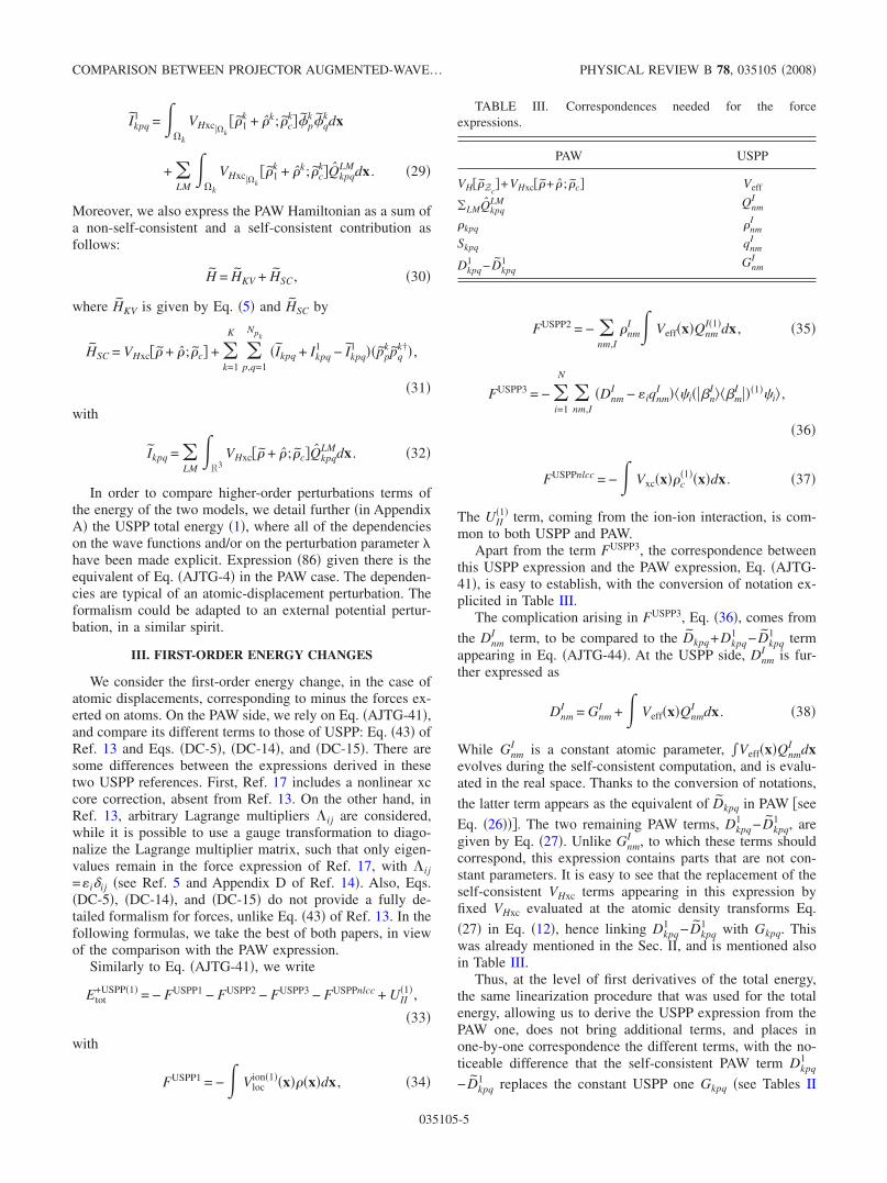
mon to both USPP and PAW.Apart from the term FUSPP3, the correspondence between

this USPP expression and the PAW expression, Eq. �AJTG-41�, is easy to establish, with the conversion of notation ex-plicited in Table III.

The complication arising in FUSPP3, Eq. �36�, comes from

the DnmI term, to be compared to the Dkpq+Dkpq

1 − Dkpq1 term

appearing in Eq. �AJTG-44�. At the USPP side, DnmI is fur-

ther expressed as

DnmI = Gnm

I + Veff�x�QnmI dx . �38�

While GnmI is a constant atomic parameter, Veff�x�Qnm

I dxevolves during the self-consistent computation, and is evalu-ated in the real space. Thanks to the conversion of notations,

the latter term appears as the equivalent of Dkpq in PAW �see

Eq. �26��. The two remaining PAW terms, Dkpq1 − Dkpq

1 , aregiven by Eq. �27�. Unlike Gnm

I , to which these terms shouldcorrespond, this expression contains parts that are not con-stant parameters. It is easy to see that the replacement of theself-consistent VHxc terms appearing in this expression byfixed VHxc evaluated at the atomic density transforms Eq.

�27� in Eq. �12�, hence linking Dkpq1 − Dkpq

1 with Gkpq. Thiswas already mentioned in the Sec. II, and is mentioned alsoin Table III.

Thus, at the level of first derivatives of the total energy,the same linearization procedure that was used for the totalenergy, allowing us to derive the USPP expression from thePAW one, does not bring additional terms, and places inone-by-one correspondence the different terms, with the no-ticeable difference that the self-consistent PAW term Dkpq

1

− Dkpq1 replaces the constant USPP one Gkpq �see Tables II

TABLE III. Correspondences needed for the forceexpressions.

PAW USPP

VH��Zc�+VHxc��+ � ; �c� Veff

�LMQkpqLM Qnm

I

�kpq �nmI

Skpq qnmI

Dkpq1 − Dkpq

1 GnmI


035105-5

and III�. As Dkpq1 − Dkpq

1 are available from the prior ground-state calculation, there is no additional computation to bedone at the level of forces.

IV. FIRST-ORDER WAVE FUNCTION CHANGE

While first-order derivatives of total energy do not rely onthe knowledge of first-order wave functions, the latter will beneeded for second-order derivatives of the total energy. Wegive in this section the correspondences for such first-orderwave function changes, which appear in Ref. 17, namely,��i and ��i. Concerning the latter notations, we suppress the exponent because we deal here only with one specificperturbation. Let us also recall that we consider nonmetallicsystems and atomic-displacement perturbations.

In the case of nonmetallic systems, wave functionchanges are not uniquely defined, as explained in AppendixD of Ref. 14. Due to the gauge freedom, the part of the wavefunction change that belongs to the occupied state manifoldhas some arbitrariness. Of course, the final expressions forenergy derivatives should be unaffected by the gauge choice.While Dal Corso17 worked naturally with the diagonal gauge�the natural choice for a formalism valid for metals as well asfor insulators�, the parallel gauge is the method of choice forinsulators, as used in our previous work.14

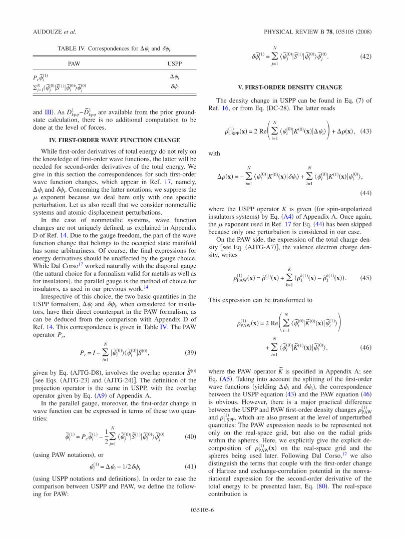
Irrespective of this choice, the two basic quantities in theUSPP formalism, ��i and ��i, when considered for insula-tors, have their direct counterpart in the PAW formalism, ascan be deduced from the comparison with Appendix D ofRef. 14. This correspondence is given in Table IV. The PAWoperator Pc,

Pc = I − �i=1

N

��i�0��i

�0��S�0�, �39�

given by Eq. �AJTG-D8�, involves the overlap operator S�0�

�see Eqs. �AJTG-23� and �AJTG-24��. The definition of theprojection operator is the same in USPP, with the overlapoperator given by Eq. �A9� of Appendix A.

In the parallel gauge, moreover, the first-order change inwave function can be expressed in terms of these two quan-tities:

�i�1� = Pc�i

�1� −1

2�j=1

N

�� j�0��S�1��i

�0�� j�0� �40�

�using PAW notations�, or

�i�1� = ��i − 1/2��i �41�

�using USPP notations and definitions�. In order to ease thecomparison between USPP and PAW, we define the follow-ing for PAW:

��i�1� = �

j=1

N

�� j�0��S�1��i

�0�� j�0�. �42�

V. FIRST-ORDER DENSITY CHANGE

The density change in USPP can be found in Eq. �7� ofRef. 16, or from Eq. �DC-28�. The latter reads

�USPP�1� �x� = 2 Re�

i=1

N

��i�0��K�0��x��i�� + ��x� , �43�

with

��x� = − �i=1

N

��i�0��K�0��x��i� + �

i=1

N

��i�0��K�1��x��i

�0�� ,

�44�

where the USPP operator K is given �for spin-unpolarizedinsulators systems� by Eq. �A4� of Appendix A. Once again,the exponent used in Ref. 17 for Eq. �44� has been skippedbecause only one perturbation is considered in our case.

On the PAW side, the expression of the total charge den-sity �see Eq. �AJTG-A7��, the valence electron charge den-sity, writes

�PAW�1� �x� = ��1��x� + �

k=1

K

��1k�1��x� − �1

k�1��x�� . �45�

This expression can be transformed to

�PAW�1� �x� = 2 Re�

i=1

N

��i�0��K�0��x��i

�1��+ �

i=1

N

��i�0��K�1��x��i

�0�� , �46�

where the PAW operator K is specified in Appendix A; seeEq. �A5�. Taking into account the splitting of the first-orderwave functions �yielding ��i and ��i�, the correspondencebetween the USPP equation �43� and the PAW equation �46�is obvious. However, there is a major practical differencebetween the USPP and PAW first-order density changes �PAW

�1�

and �USPP�1� , which are also present at the level of unperturbed

quantities: The PAW expression needs to be represented notonly on the real-space grid, but also on the radial gridswithin the spheres. Here, we explicitly give the explicit de-composition of �PAW

�1� �x� on the real-space grid and thespheres being used later. Following Dal Corso,17 we alsodistinguish the terms that couple with the first-order changeof Hartree and exchange-correlation potential in the nonva-riational expression for the second-order derivative of thetotal energy to be presented later, Eq. �80�. The real-spacecontribution is

TABLE IV. Correspondences for ��i and ��i.

PAW USPP

Pc�i�1� ��i

� j=1N �� j

�0��S�1��i�0�� j

�0� ��i


035105-6

�� + ��1��x�

= 2 Re�i=1

N

�i�0��x�Pc�i

�1��x� + �k=1

K

�p,q=1

Npk

�LM

QkpqLM�0��x�

��i=1

N

�i�0��pp

k pqk†��0��Pc�i

�1�� + �� + ��x� , �47�

with

�� + ��x�

= − Re�i=1

N

�i�0��x��i

�1��x� + �k=1

K

�p,q=1

Npk

�LM

QkpqLM�0��x�

��i=1

N

��i�0��pp

k pqk†��0��i

�1��+ �

k=1

K

�p,q=1

Npk

�LM

�i=1

N

�QkpqLM�1��x��i

�0��ppk pq

k†��0��i�0��

+ QkpqLM�0��x��i

�0��ppk pq

k†��1��i�0�� . �48�

The first �all-electron� sphere contribution is

�1k�1��x� = 2 Re �

p,q=1

Npk

�i=1

N

�pk�x��q

k��x��i�0��pp


�1��+ ��1

k�x� �49�

with

��1k�x� = �

p,q=1

Npk

�i=1

N

�pk�x��q

k��x��− Re��i�0��pp


�1��

+ ��i�0��pp


�0�� , �50�

and the second �pseudized� sphere contribution is

��1k + �k��1��x� = 2 �

p,q=1

Npk

�i=1

N

�pk�x��q

k��x� + �LM

QkpqLM�0��x��

�Re��i�0��pp


�1��

+ ��1k + �k��x� �51�

with

��1k + �k��x� = �

p,q=1

Npk

�i=1

N

�pk�x��q

k��x� + �LM


� �− Re��i�0��pp


�1��

+ ��i�0��pp


�0��

+ �p,q=1

Npk

�LM


i=1

N

�i�0��pp


�0�� .

�52�

VI. FIRST-ORDER HAMILTONIAN AND POTENTIALCHANGES

In the USPP formalism, the Sternheimer equation, Eq.�DC-29�, writes

�H�0� − �i�0�S�0��i� = − Pc

†�VKS�1� − �i

�0�S�1��i�0�� , �53�

where the unperturbed Hamiltonian H�0� is given by Eq.�A11� of Appendix A, while in the PAW case �see Eq.�AJTG-73� and Appendix D of Ref. 14� we have

Pc†�H�0� − �i

�0�S�0��Pc�i�1�� = − Pc

†�H�1� − �i�0�S�1��i

�0�� ,

�54�

with direct correspondences of the different terms in theseequations.

We give now the first-order changes of the Hamiltonianoperator, which appear in the Sternheimer equations and fur-ther in Sec. VII. In the USPP case, Dal Corso started fromEqs. �21� and �22�, and distinguished a first-order partial de-rivative of VKS as follows:

H�1� = VKS�1� =

�VKS

�+ VHxc

�1� , �55�

with

�VKS

�=

�VNLUSPP

�+ �Vloc

ion

�K + Veff

�K

�. �56�

Note that�VKS

� is not a true partial derivative of VKS withrespect to : There are direct dependencies of VHxc on thatare not mediated by wave function changes, see Appendix A.The definition given by Dal Corso corresponds actually to apartial derivative at fixed VHxc. In order to make the notationclear, we will add in several equations that follow, whenappropriate, a subscript VHxc

�0� to indicate that the Hamiltonianoperator is derived under the hypothesis that VHxc=VHxc

�0� .

Coming now to PAW, the first-order change of H, see Eq.

�AJTG-18�, might be given in term of HKV�1� and HSC

�1�. For

phonons, the equation describing HKV�1� , Eq. �AJTG-B2�, sim-

plifies somewhat

HKV�1� = VH��Zc

�1�� + �k=1

K

�p,q=1

Npk

�Ekpq�0� �pp

k pqk†��1� + Ekpq

�1� �ppk pq

k†��0�� ,

�57�

with

Ekpq�1� = �

LM

R3VH��Zc

�1��QkpqLM�0� + VH��Zc

�0��QkpqLM�1�dx

− �LM

�k

VH��k��Zc

�1��QkpqLM�0�dx

+ ��pk �VH��k�

��Zc

k�1��qk�k − ��p

k �VH��k��Zc

k�1��qk�k.

Thanks to Eq. �57�, one can see that HKV�1� corresponds to the

following USPP expression:


035105-7

�VNLUSPP

�+ �Vloc

ion

�K + Vloc

ion�K

�. �58�

The comparison with USPP is based on the following de-

composition of H:

H�1� = � �H

��

VHxc�0�

+ VHxc�1� , �59�

with

� �H

��

VHxc�0�

= HKV�1� + �

k=1

K

�p,q=1

Npk

��ppk pq

k†��0�R3

VHxc�� + �; �c��0��LM

QkpqLM�1�dx

+ �ppk pq

k†��1�R3

VHxc�� + �; �c��0��LM

QkpqLM�0�dx

+ �ppk pq

k†��1��k

VHxc��1k ;�c

k��0��pk�q

kdx

− �ppk pq

k†��1��k

VHxc��1k + �k; �c

k��0�

��pk�q

k + �LM

QkpqLM�0��dx� . �60�

The last two terms of Eq. �60�, which include an integrationover the spheres, are not present in the USPP formalism. Allthe other contributions to this PAW expression have theircounterpart in the USPP formalism.

Also,

VHxc�1� = VHxc�� + �; �c��1� + �

k=1

K

�p,q=1

Npk

�ppk pq

k†��0�

�R3

VHxc�� + �; �c��1��LM

QkpqLM�0�dx

+ �k

VHxc��1k ;�c


kdx

− �k


k��1�

��pk�q

k + �LM


The last two terms of Eq. �61�, which include an integrationover the spheres, are not present in the USPP formalism.

VII. NONVARIATIONAL SECOND-ORDER ENERGYCHANGES

In this section, we detail the different steps needed toestablish the correspondences for the second-order change ofthe energy, for nonmetallic systems and atomic displace-

ments, as before. First of all, let us recall the expressions ofthe second-order energy in both models. They are obtainedfrom

Etot,nonvar+�2� =

1

2 d

dEtot

+�1��i�0� + ��1��

�=0�. �62�

In the USPP case, this expression corresponds to the half-sum of Eq. �DC-35� and also of Eqs. �DC-39�–�DC-42��taken with one parameter, i.e., = in the notations usedtherein, and for nonmetallic systems�. Explicitly, the USPPexpression is given by

1

2

d2

d2Etot,notvar+USPP = EUSPP1 + EUSPP2 + EUSPP3 + EUSPP4 + EUSPP5

+ UII�2�, �63�

with

EUSPP1 =1

2�i=1

N

��i�0��

�2VKS

�2 − �i�0� �2S

�2 ��i�0�� 64�

�see Eq. �DC-39��,

EUSPP2 = �i=1

N

��i��VKS

�− �i

�0� �S

��i

�0�� 65�

�see Eq. �DC-40��,

EUSPP3 =1

2 VHxc

�1� �x��x�dx �66�

�see Eq. �DC-41��, where �� is given by Eq. �44�,

EUSPP4 = − �i=1

N

��i��VKS

�− �i

�0� �S

��i

�0�� 67�

�see Eq. �DC-42��,

EUSPP5 =1

2 Vxc

�1��c

�+ Vxc

�0��2�c

�2 ��x�dx �68�

�see Eq. �DC-35��.In the PAW case, the nonvariational second-order energy

perturbation writes as follows �see Eq. �AJTG-80��:

Etot,notvar+PAW�2� = �

i=1

N

��i�1��HKV

�1� − �i�0�S�1��i

�0��

+ ��i�0��HKV

�2� − �i�0�S�2��i

�0��

−1

2 �j,j�=1

N

� j j��1�� j

�0��S�1�� j��0��

+ EHxc0�2:2� + EHxc0

�2:1,1� + U�2�, �69�

where the external potential is neglected. The terms EHxc0�2:2�

and EHxc0�2:1,1� are specified in Appendix B. It is shown there that

they can be split as


035105-8

EHxc0�2:1,1� = EHxc0,v

�2:1,1� + EHxc0,c�2:1,1� �70�

and

EHxc0�2:2� = EHxc0,v0

�2:2� + EHxc0,v1�2:2� + EHxc0,c

�2:2� , �71�

where the subscript c indicates terms that correspond to xc

core corrections. HKV�2� is also specified in Appendix B.

The grouping of terms in the PAW formalism of Ref. 14can be reworked, to make the same grouping in the USPPformalism of Ref. 17 appear. We will obtain

1

2

d2

d2Etot,notvar+PAW = EPAW1 + EPAW2 + EPAW3 + EPAW4 + EPAW5

+ UII�2�, �72�

in term-by-term analogy with Eq. �69�. However, several of

these terms will contain additional contributions, comingfrom the variations of quantities in the PAW spheres, notpresent in the USPP case.

The term EPAW1 is obtained as follows:

EPAW1 = �i=1

N


�2� − �i�0�S�2��i

�0�� + EHxc0,v0�2:2�

=1

2�i=1

N

��i�0�� 2H

�2�VHxc

�0�− �i

�0� �2S

�2 ��i�0�� , �73�

where �1 /2��2S /�2�= S�2� and

1

2��2H

�2�VHxc

�0�= HKV

�2� + �k=1

K

�p,q=1

Npk �ppk pq

k†��0�R3

VHxc�� + �; �c��0��LM

QkpqLM�2�dx + �pp

k pqk†��1�

R3VHxc�� + �; �c��0��

LM

QkpqLM�1�dx

+ �ppk pq

k†��2�R3

VHxc�� + �; �c��0��LM

QkpqLM�0�dx + �pp

k pqk†��2�

�k

VHxc��1k ;�c


kdx

− �ppk pq

k†��2��k



k + �LM


The last two terms of Eq. �74�, which include an integration over the spheres, are not present in the USPP formalism. All theother contributions to this PAW expression have their counterpart in the USPP formalism.

The terms EPAW2 and EPAW4 write, respectively,

EPAW2 = �i=1

N

�Pc�i�1�� H

��

VHxc�0�

− �i�0� � S

��i

�0�� 75�

and

EPAW4 = − �i=1

N

��i�1�� H

��

VHxc�0�

− �i�0� � S

��i

�0�� , �76�

where �S /�= S�1� and �H /��VH=c�0� is given by Eq. �60�.

EPAW2 and one-half of EPAW4 originate from Eq. �69� in the following combination:

�i=1

N


�1� − �i�0�S�1��i

�0�� + EHxc0,v1�2:2� = �

i=1

N

��i�1��H

��

VHxc�0�

− �i�0� � S

��i

�0��

= �i=1

N

�Pc�i�1� −

1

2��i

�1��H

��

VHxc�0�

− �i�0� � S

��i

�0�� = EPAW2 +1

2EPAW4. �77�

The other half of EPAW4 is to be found in the term − 12� j,j�=1

N � j j��1�� j

�0��S�1�� j��0�� of Eq. �69�. We develop the first-order

Lagrange multipliers � j j��1�, Eq. �AJTG-81�, with the Kohn–Sham equation, Eq. �24�, and use the expression of the first-order

wave functions in the parallel gauge, Eq. �40�, as follows:

� j j��1� = �� j�

�0��H�1� −�� j

�0� + � j��0��

2S�1�� j

�0�� . �78�


035105-9

As outlined previously, H�1�, present in this equation, differs from �H� needed in EPAW4.

We now use the splitting of Eq. �59�, whose first term in Eq. �78� gives precisely the other half of EPAW4 as follows:

−1

2 �j,j�=1

N

�� j��0�� H

��

VHxc�0�

−�� j

�0� + � j��0��

2S�1�� j

�0�� j�0��S�1�� j�

�0��

= −1

2 �j,j�=1

N

�� j��0�� H

��

VHxc�0�

− � j�0�S�1�� j

�0�� j�0��S�1�� j�

�0��

= −1

2�j=1

N

�� j�1�� H

��

VHxc�0�

− � j�0� � S

�� j

�0��

=1

2EPAW4. �79�

The term EPAW3 comes from the remaining VHxc�1� contribu-

tion to Eq. �78�, and from EHxc0,v�2:1,1� . After some manipulation,

one gets

EPAW3 =1

2

R3VHxc

�1� �x�� + ��x�dx

+1

2�k=1

K �k

�VHxc��1k ;�c

k��1��1k�x�dx

−1

2�k=1

K �k

�VHxc��1k + �k; �c

k��1��1k + �k��x�dx .

�80�

In this third PAW contribution, the difference with the USPPexpressions is the biggest: Not only the last two terms, to beevaluated on the spherical grid, have appeared, but such ad-

ditional contributions are also present in VHxc�1� and ��x�, see

Eqs. �48� and �61�.The last contributions to the nonvariational second-order

derivatives of the total energy come from the core chargechanges as follows:

EPAW5 = EHxc0,c�2:1,1� + EHxc0,c

�2:2� = R3

1

2Vxc�� + � + �c��1��c

�1�

+ Vxc�� + � + �c��0��c�2�dx �81�

This expression is the same in the USPP and PAW formal-isms.

To summarize this section, we have seen that the differentterms contributing to the nonvariational second-energy de-rivative of the total energy, as formulated by Dal Corso inRef. 17, have their counterpart in the PAW formalism, de-rived from Ref. 14 after some manipulation, with the bigdifference that several integrals over the real space are to beaugmented by integral over the spheres: EPAW3, see Eq. �80�;EPAW5, see Eq. �81�; and � �2H

�2 �VHxc�0� present in Eq. �73�, see Eq.

�74�.Although the present derivation has been made only for

insulators, it generalizes straightforwardly to the case of met-als. Indeed, we note that the similarities between the USPPand PAW are strong enough to leave unchanged the keystructure where the differences between insulators and met-als appear, namely, the definition of the first-order wavefunction changes, and the definition of the Sternheimer equa-tion. Hence, the more complete treatment of perturbationtheory by Dal Corso, which includes the case of metals andvarying occupation numbers, can be incorporated readily,without changes, into the present formalism. This can bethought the other way around: It is possible to incorporate inthe formalism by Dal Corso, localized modifications, tochange it from USPP to PAW. By the same token, the gen-eralization from one perturbation to two perturbations, alsotreated by Dal Corso, is straightforward.

VIII. VARIATIONAL SECOND-ORDER ENERGYCHANGES

A variational formulation for the PAW second-order en-ergy changes has also been written in Ref. 14, see Eq. �DC-67�. In this reference, the first-order wave function changewas not split into the two components that appear naturallyin the actual software implementation, ��i and ��i. Also, thetechnique used in the USPP formalism, namely, to isolatederivatives of the Hamiltonian at fixed Hartree andexchange-correlation potential yields a more compact ex-pression than in Ref. 14. We will now treat these two modi-fications of the original PAW result.

Let us start with the latter, where we take advantage of thedifferent definitions presented here. Ignoring the explicitchange of external potential, which was included in Ref. 14,we find


035105-10

Etot+PAW�2� = min

�i�1��

i=1

N ��i�1��H − �iS��0��i

�1��

+ ��i�0�� H

��

VHxc�0�

− �i�0�S�1��i

�1�� + �c.c.��+ EHxc

�2:1,1�� + EPAW1 + EHxc0,c�2:2� + UII

�2�. �82�

The splitting of �i into a varying part, ��i, and a fixedpart, ��i, allows us to make more apparent the variationalcharacter of Etot

+PAW�2�. One benefits also from the followingidentity �valid for insulators�:

�i=1

N

��i�1��H − �iS��0��i

�1�� = �i=1

N

�Pc�i�1��H − �iS��0��Pc�i

�1�� ,

�83�

giving

Etot+PAW�2� = min

Pc�i�1��

i=1

N ��Pc�i�1��H − �iS��0��Pc�i

�1��

+ ��i�0�� H

��

VHxc�0�

− �i�0�S�1��Pc�i

�1�� + �c.c.��+ EHxc

�2:1,1�� + EPAW1 + EPAW4 + EHxc0,c�2:2� + UII

�2�.

�84�

The equivalent formula for the USPP formalism writes

Etot+USPP�2� = min

��i��

i=1

N ��i��H − �iS��0��i�

+ ��i�0��

�VKS

�− �i

�0� �S

��i� + �c.c.��

+1

2 VHxc

�1� �x��1��x�dx +1

2 Vxc

�1��x��c

��x�dx�

+ EUSPP1 + EUSPP4 +1

2 Vxc

�0��x��2�c

�2 �x�dx + UII�2�.

�85�

Equations �84� and �85� might be used to determine theset of first-order wave functions, and associated first-orderchanges of density and potential, as an alternative to theSterheimer equation approach. A conjugate-gradient algo-rithm has been proposed in Ref. 20 for such purpose. Notealso that for the specific case of the electric field perturbationand derivative of the wave functions with respect to the wavevector, variational USPP expressions had been presented inRef. 18.

IX. CONCLUSIONS AND PERSPECTIVES

The density-functional perturbation theory, taken withnorm-conserving pseudopotentials, leads to expressions thatcontain numerous terms. Still, their complexity is not toolarge, and one can gain confidence in the final implementa-tion in a real software; thanks to well chosen references buildfrom finite differences of adequate expressions.

If the USPP or PAW are used instead of norm-conservingpseudopotentials, the complexity of the formalism explodes,and the number of finite-difference quantities to be con-structed becomes much larger. In order to gain confidence inthe final expressions obtained in PAW14 and USPP,17 and intheir implementation, even before painful finite-differencetesting, we have established the correspondence between thefinal results in USPP and PAW. These formalisms are rathersimilar at the level of nonperturbed density-functional theory,although not identical. We have recalled the existing differ-ences at that level, the USPP being derived from the PAW;thanks to a linearization of the Hartree and exchange-correlation contribution inside the atomic spheres, around theatomic reference. The correspondence between the results ofthe two above-mentioned papers is harder to establish whenworking with first- or second-order derivatives: There existsnumerous degrees of freedom to rearrange the terms. At eachstage, we have established the correspondences betweenquantities, and highlighted the operational similarity or dif-ference of terms, and the physical similarity or difference.

In the PAW case, numerous additional contributions arepresent, all arising from the appearance of integrals over theatomic PAW spheres �one for the all-electron quantities, andone for the pseudized quantities�, while only integrals overthe real space are present in the USPP formalism. Althoughour derivation was restricted to the case of insulators, and foronly one perturbation, the generalization of the nonvaria-tional second-order energy changes to the case of metals, andto two types of perturbations taken together is straightfor-ward. Indeed, for this expression examined in its full gener-ality by Dal Corso in Ref. 17, the modifications going fromUSPP to PAW have such a regular structure that they do notinfluence the modifications needed to go from insulators tometals and from one to two perturbations.

The variational expression for the second-order energychanges has also been examined in the present paper. Wehave taken into account the splitting of the first-order wavefunction in two parts �projection outside of the treated space,and remainder�, to provide a formula closer to implementa-tion than the previously published PAW one. Its reduction tothe USPP case has also been proposed.

It was pointed out by Kresse and Joubert10 that the USPPmethod is generally as reliable as the PAW method, exceptfor magnetic systems. It remains to be studied whether thesame conclusion holds at the level of the second-order de-rivatives of the energy.

ACKNOWLEDGMENTS

One of the authors �X.G.� would like to acknowledge fi-nancial support by the Interuniversity Attraction Poles Pro-gram �Grant No. P6/42�—Belgian State—Belgian Science


035105-11

Policy, the Communaute Francaise de Belgique �Action deRecherches Concertee, Grant No. 07/12-003�, and the Euro-pean Union �Grant No. NMP4-CT-2004–500198, “NANO-QUANTA” Network of Excellence “Nanoscale QuantumSimulations for Nanostructures and Advanced Materials,”and “ETSF” Integrated Infrastructure Initiative�.

APPENDIX A: DEPENDENCIES OF THE UNPERTURBEDULTRASOFT PSEUDOPOTENTIAL TOTAL ENERGY

We give here an expression of the unperturbed USPP totalenergy, in which the �corresponding to an atomic displace-ment� and/or �i dependencies of all the different physicalquantities have been made explicit. This expression has to becompared with Eq. �AJTG-4� given in the PAW case. Thedependencies occur in the following way:

Etot+USPP��i,� = �

i=1

N

��i� −1

2�2 + VNL��i�

+ EHxc��i,�;�c�� + Vlocion��i,�dx

+ UII�� − �i,j=1

N

�ij��i,��i�S�� j� − �ij� .

�A1�

The Hartree and exchange-correlation term is defined by

EHxc��i,�;�c�� = EH��i,�� + Exc��i,� + �c��A2�

with

��x��i,� = �i=1

N

��i�K�x��i� , �A3�

and

K�x�� = K�x;x1,x2��

= ��x − x1��x − x2�

+ �nm,I

QnmI �x��n

I �x1��mI†�x2�� . �A4�

The previous operator, associated with the USPP ��i ,�,corresponds to the development of the PAW quantity ��i�+ ��i ,�. The corresponding PAW operator is defined by

K�x�� = K�x;x1,x2�� = ��x − x1��x − x2�

+ �k=1

K

�p,q=1

Npk

�LM

QkpqLM�x��pp

k�x1�pqk†�x2�� .

�A5�

The nonlocal part of the U.S. pseudopotential is given by

VNL�� = �nm,I

GnmI ��n

I �mI†�� . �A6�

This relation is operationally equivalent to the PAW case,which consists in

�k=1

K

�p,q=1

Npk

Ekpq� �ppk pq

k†�� A7�

with Ekpq� given by Eq. �19�.Moreover, the N2 constraints on the wave functions �i

�see Eq. �DC-7��

��i�S�� j� − �ij = 0 �A8�

correspond to the Eq. �AJTG-5� in the PAW case. The USPPoverlap operator

S�� = I + �nm,I

qnmI ��n

I �mI†�� A9�

with qnmI = Qnm

I �x�dx has to be compared with Eq. �AJTG-23�. The structure of the overlap operator is the same in bothmodels, with a different definition of the coefficients �seeTable III for the correspondences of qnm

I and QnmI �.

Lastly, the Lagrange multipliers that guarantee the fulfill-ment of the constraints are given by the following relations:

�ij��i,� = ��i�H��i,�� j� , �A10�

where the USPP Hamiltonian has the following dependencies�to be compared to Eq. �AJTG-18��:

H��i,� = −1

2�2 + Veff��i,� + VNL��

+ �nm,I

Veff��i,�QnmI ��n

I �mI†�� ,

�A11�

with

Veff��i,� = Vlocion�� + VHxc��i,�;�c�� . �A12�

Let us finally mention the KS potential, defined by

VKS��i,� = VNL�� + R3

Veff�x��i,�K�x��dx .

�A13�

APPENDIX B: ADDITIONAL EXPRESSIONS NEEDEDFOR THE SECOND-ORDER ENERGY COMPARISON

We develop here some expressions that are useful tohandle the comparison of the second-order perturbation of

the total energy: EUSPP3 in the USPP case, and EHxc0�2:1,1�, EHxc0

�2:2� ,and Ekpq

�2� in the PAW framework.In the USPP case, EUSPP3 �see Eq. �66�� writes, thanks to

Eq. �44� given for ��, as follows:

EUSPP3 = −1

2�i=1

N VHxc�1� �i

�0��idx �B1�

−1

2�i=1

N

�n,m,I

��i�0��m

I�0��nI�0��i� VHxc

�1� QnmI�0�dx

�B2�


035105-12

+1

2�i=1

N

�n,m,I

��i�0��m

I ��nI ��0��i

�0�� VHxc�1� Qnm

I�1�dx

�B3�

+1

2�i=1

N

�n,m,I

��i�0��m

I ��nI ��1��i

�0�� VHxc�1� Qnm

I�0�dx .

�B4�

From the PAW point of view, EHxc0�2:1,1� �see Eq. �AJTG-E2��

is given by

EHxc0�2:1,1� = EHxc0,v

�2:1,1� + EHxc0,c�2:1,1� , �B5�

with a valence contribution �linear in �i�1�� corresponding to

Eq. �B3� and Eq. �B4� as follows:

EHxc0,v�2:1,1� =

1

2�k=1

K

�p,q=1

Npk

�LM

�kpq�0�

R3�VHxc�� + �; �c��1�Qkpq

LM�1�dx

+1

2�k=1

K

�p,q=1

Npk

�LM

�kpq�1�

R3�VHxc�� + �; �c��1�Qkpq

LM�0�dx

+1

2�k=1

K

�p,q=1

Npk

�kpq�1�

�k

�VHxc��1k ;�c


kdx

−1

2�k=1

K

�p,q=1

Npk

�kpq�1�

�k

�VHxc��1k + �k; �c


k

+ QkpqLM�0��dx , �B6�

and a core charge contribution

EHxc0,c�2:1,1� =

1

2

R3�Vxc�� + �; �c��1��c

�1�dx

+1

2�k=1

K �k

�Vxc��1k + �c

k��1��ck�1�dx

−1

2�k=1

K �k

�Vxc��1k + �k + �c

k��1��ck�1�dx . �B7�

Besides, the term EHxc0�2:2� �see Eq. �AJTG-E1�� is defined by

EHxc0�2:2� =

R3VH�� + ��0��0

�2�dx

+ �k=1

K �k

VH��1k�0��1

�2:1� + �1�2:0��dx �B8a�

− �k=1

K �k

VH��1 + ��k�0��1�2:1� + �1

�2:0� + �0�2��dx

�B8b�

+ R3

Vxc�� + � + �c��0��0�2� + �c

�2��dx

+ �k=1

K �k

Vxc��1k + �c

k��0��1�2:1� + �1

�2:0� + �ck�2��dx

�B8c�

− �k=1

K �k

Vxc��1k + �k + �c

k��0��1�2:1� + �1

�2:0� + �0�e2�

+ �ck�2��dx . �B8d�

The different contributions of the second-order changes ofthe densities �1 and �1 are given in Appendix C of Ref. 14and �0

�2� by Eq. �E3� of the same reference. For the compari-son of the second-order energy, some additional manipula-tions are useful. First, we gather the terms involving corecharge densities in Eqs. �B8c� and �B8d� leading to the fol-lowing terms:

EHxc0,c�2:2� =

R3Vxc�� + � + �c��0��c

�2�dx

+ �k=1

K �k

Vxc��1k + �c

k��0��ck�2�dx

− �k=1

K �k

Vxc��1k + �k + �c

k��0��ck�2�dx , �B9�

EHxc0�2:2� − EHxc0,c

�2:2� = R3

VHxc�� + �; �c��0��0�2�dx

+ �k=1

K �k

VHxc��1k ;�c

k��0��1�2:1� + �1

�2:0��dx

− �k=1

K �k


k��0��1�2:1� + �1

�2:0�

+ �0�2��dx . �B10�

Then, the development of the different second-order changesof the densities �1 , �1 and �0 �see Appendix C and Eq. �E3�of Ref. 14 for the corresponding expressions� in Eqs. �B8a�,�B8b�, and �B10� yields the following valence terms:

EHxc0,v0�2:2�

= �i=1

N

��i�0��

R3VHxc�� + ��0�; �c

�0��K�2�dx��i�0��

+ �i=1

N

��i�0��

k=1

K �k

VHxc��1k + �k��0�;�c

k�0��K�2�dx��i�0��


035105-13

− �i=1

N

��i�0��

k=1

K �k

VHxc��1k + �k��0�; �c

k�0��K�2�dx��i�0�� ,

�B11�

which depends on �i�0� only, and

EHxc0,v1�2:2�

= �i=1

N

��i�1��

R3VHxc�� + ��0�; �c

�0��K�1�dx��i�0��

+ �i=1

N

��i�1��

k=1

K �k

VHxc��1k + �k��0�; �c

k�0��K�1�dx��i�0��

− �i=1

N

��i�1��

k=1

K �k

VHxc��1k + �k��0�; �c

k�0��K�1�dx��i�0��

�B12�

which involves also first-order changes �i�1�. In that way, the

previous manipulations lead us to split EHxc0�2:2� into three con-

tributions, a core term on one side and two valence terms, onthe other side:

EHxc0�2:2� = EHxc0,c

�2:2� + EHxc0,v0�2:2� + EHxc0,v1

�2:2� . �B13�

The expression of HKV�2� is given in Eq. �AJTG-B4�. It uses

the coefficients Ekpq�2� that are somewhat simplified with re-

spect to the expression �AJTG-B5� for a perturbation of thephonon type, as follows:

Ekpq�2� = �

LM

R3VH��Zc

�2��QkpqLM�0� + VH��Zc

�1��QkpqLM�1�

+ VH��Zc

�0��QkpqLM�2�dx − �

LM

�k

VH��k��Zc

�2��QkpqLM�0�dx�

+ ��pk �VH��k�

��Zc

k�2��qk�k − ��p

k �VH��k��Zc

k�2��qk�k.

�B14�

1 See, e.g., R. Martin, Electronic Structure: Basic Theory andPractical Methods �Cambridge University Press, Cambridge,2004�.

2 S. Baroni, P. Giannozzi, and A. Testa, Phys. Rev. Lett. 58, 1861�1987�.

3 For a review, see S. Baroni, S. de Gironcoli, A. Dal Corso, and P.Giannozzi, Rev. Mod. Phys. 73, 515 �2001�.

4 For a recent primer, see X. Gonze, G.-M. Rignanese, and R.Caracas, Z. Kristallogr. 220, 458 �2005�.

5 X. Gonze, Phys. Rev. A 52, 1096 �1995�; 54, 4591�E� �1996�.6 D. Vanderbilt, Phys. Rev. B 41, 7892 �1990�.7 The PWSCF/PHONON software, which implements DFPT for

norm-conserving pseudopotentials as well as ultrasoft pseudopo-tentials, is available at http://www.pwscf.org; It is a part of theQUANTUM-ESPRESSO package, see S. Scandolo, P. Giannozzi, C.Cavazzoni, S. de Gironcoli, A. Pasquarello, and S. Baroni, Z.Kristallogr. 220, 574 �2005�.

8 The ABINIT software, which implements DFPT for norm-conserving pseudopotentials, and soon for PAW, is available athttp://www.abinit.org; See X. Gonze, J.-M. Beuken, R. Caracas,F. Detraux, M. Fuchs, G.-M. Rignanese, L. Sindic, M. Verstra-ete, G. Zerah, F. Jollet, M. Torrent, A. Roy, M. Mikami, Ph.Ghosez, J.-Y. Raty, and D.C. Allan. Comput. Mater. Sci. 25, 478�2002�; X. Gonze, G.-M. Rignanese, M. Verstraete, J.-M. Beu-ken, Y. Pouillon, R. Caracas, F. Jollet, M. Torrent, G. Zerah, M.Mikami, Ph. Ghosez, M. Veithen, J.-Y. Raty, V. Olevano, F.Bruneval, L. Reining, R. Godby, G. Onida, D. R. Hamann, and

D. C. Allan, Z. Kristallogr. 220, 558 �2005�.9 P. E. Blöchl, Phys. Rev. B 50, 17953 �1994�.

10 G. Kresse and D. Joubert, Phys. Rev. B 59, 1758 �1999�.11 N. A. W. Holzwarth, G. E. Matthews, R. B. Dunning, A. R.

Tackett, and Y. Zeng, Phys. Rev. B 55, 2005 �1997�.12 M. Torrent, F. Jollet, F. Bottin, G. Zérah, and X. Gonze, Comput.

Mater. Sci. 42, 337 �2008�.13 K. Laasonen, A. Pasquarello, R. Car, C. Lee, and D. Vanderbilt,

Phys. Rev. B 47, 10142 �1993�.14 C. Audouze, F. Jollet, M. Torrent, and X. Gonze, Phys. Rev. B

73, 235101 �2006�.15 X. Gonze, Phys. Rev. A 52, 1086 �1995�.16 A. Dal Corso, A. Pasquarello, and A. Baldereschi, Phys. Rev. B

56, R11369 �1997�.17 A. Dal Corso, Phys. Rev. B 64, 235118 �2001�.18 P. Umari, X. Gonze, and A. Pasquarello, Phys. Rev. B 69,

235102 �2004�.19 We choose to follow the notation of Kresse and Joubert �Ref.

10�, which is more convenient for a comparison with PAW co-efficients in the present paper. Indeed, this notation avoids con-fusion with the notation �0� used for DFPT, as we consider un-perturbed quantities in Sec. II. Let us also mention that we donot consider the species to which each atom belongs, for thesake of simplicity, avoiding the notation ��I�.

20 X. Gonze, D. C. Allan, and M. P. Teter, Phys. Rev. Lett. 68,3603 �1992�; X. Gonze, Phys. Rev. B 55, 10337 �1997�.


035105-14

Documents

Comparison between projector augmented-wave and ultrasoft pseudopotential formalisms at the density-functional perturbation theory level