Confined hydrogen atom by the Lagrange-mesh method: Energies, mean radii, and dynamicpolarizabilities

D. Baye1,2,* and K. D. Sen3,†

1Physique Quantique, C.P. 165/82, Université Libre de Bruxelles, B 1050 Brussels, Belgium2Physique Nucléaire Théorique et Physique Mathématique, C.P. 229, Université Libre de Bruxelles, B 1050 Brussels, Belgium

3School of Chemistry, University of Hyderabad, Hyderabad 500046, India�Received 26 May 2008; published 5 August 2008�

The Lagrange-mesh method is an approximate variational calculation which resembles a mesh calculationbecause of the use of a Gauss quadrature. The hydrogen atom confined in a sphere is studied with Lagrange-Legendre basis functions vanishing at the center and surface of the sphere. For various confinement radii,accurate energies and mean radii are obtained with small numbers of mesh points, as well as dynamic dipolepolarizabilities. The wave functions satisfy the cusp condition with 11-digit accuracy.

DOI: 10.1103/PhysRevE.78.026701 PACS number�s�: 02.70.Hm, 02.70.Jn, 31.15.ap

I. INTRODUCTION

Recent developments in nanotechnology have renewed in-terest in the modeling of spatially confined quantum systemsunder the influence of a wide variety of confining potentials.For example, the electronic properties of quantum dots arestudied by considering a set of electrons confined within aprescribed potential. Atoms and molecules confined insidehelium droplets, fullerenes, and zeolites provide further pos-sibilities of constructing spatially confined systems. For adetailed account of such applications we refer the reader torecent review articles �1–3� and references therein.

The hydrogen atom confined in an impenetrable spherewas introduced to simulate the effect of high pressure on itsstatic dipole polarizability �4�. An analytical solution interms of the confluent hypergeometric function exists, butthe energies are only implicitly given �5,6�. The spectrum ofthis system is discrete, without the accidental degeneracy ofthe free hydrogen atom. In spite of this lack of degeneracy,the levels of the confined hydrogen atom are labeled with thesame quantum numbers nl as for free hydrogen, where n− l−1 represents the number of nodes of the radial wave func-tion.

Two kinds of degeneracies are identified for the confinedstates �7–10�. They appear for special values of the radius Rof spherical confinement, corresponding to the locations ofthe radial nodes in the free hydrogen atom states with quan-tum numbers nl. For these values, the Schrödinger equationand the boundary condition are simultaneously satisfied atthe same energy as for the free atom. The confined wavefunction has one node less than the free one. This incidentaldegeneracy implies that the energy of a confined nl stateequals that of the free n+1, l state. For example, at R=2 a.u., the confined 1s state has the same energy as the 2sstate of the free H atom. Other examples of incidental degen-eracy have been discussed in the literature �11�. The simul-taneous degeneracy arises at the values R= �l+1��l+2� and issuch that a pair of confined states with quantum numbers nl

and n+1, l+2 correspond to the same energy value �7�. Forexample, at R=2 a.u., the �2s ,3d� , �3s ,4d� , . . . pairs becomedegenerate, with different energy values for each pair.

We note here that except for the incidental degeneracycases, the energy of the confined state is not analyticallyknown. A numerical resolution is thus necessary �12�. Thisproblem is a good testing ground for numerical methods be-cause the energies in Ref. �12� can be considered as exact. Inthis paper we apply the Lagrange-mesh method to such con-fined model calculations.

The Lagrange-mesh method is an approximate variationalcalculation which resembles a mesh calculation because ofthe use of a Gauss quadrature �13–16�. It provides very ac-curate results with few mesh points in a variety of quantum-mechanical problems: bound �17� and scattering �18� states,three-body atomic �19� and nuclear �20� systems, etc. Strik-ingly, its accuracy is not worse than the accuracy of thecorresponding variational calculation, performed withoutGauss approximation �15�. This accuracy on energies, radii,and several other observables is much better than the accu-racy of the Gauss quadrature on matrix elements betweenLagrange functions. For example, while scalar products ofdifferent Lagrange functions seem to vanish when calculatedwith the Gauss quadrature, they do not vanish when calcu-lated exactly. Nevertheless, the Lagrange basis functions canbe treated as an orthogonal basis without loss of accuracy.

This method has, however, the same limitations as theGauss quadrature; i.e., the accuracy disappears if the inte-grands or some of their derivatives have discontinuities. Thefirst attempts to calculate with this technique the energies ofthe simple hydrogen atom failed because of the singularity atthe origin in the Coulomb potential for s waves and in thecentrifugal and Coulomb terms for other partial waves �13�.The problem could be cured with the regularization tech-nique �14–16�: the basis functions are multiplied by somefactors aimed at removing discontinuities of the integrandswhile preserving the advantages of the Gauss quadrature.With this approach, the test with the hydrogen atom becomessuccessful.

As stated above, our aim is to apply this simple techniqueto the hydrogen atom confined in a spherical box. The basisfunctions must thus vanish at the surface of the sphere. For

*dbaye@ulb.ac.be†kalidas.sen@gmail.com

PHYSICAL REVIEW E 78, 026701 �2008�

1539-3755/2008/78�2�/026701�7� ©2008 The American Physical Society026701-1

the unconfined hydrogen atom, accurate solutions with fewmesh points are obtained with a regularized Lagrange-Laguerre basis �14–16,21�. Here we introduce a Lagrangemesh, based on shifted Legendre polynomials multiplied bya regularization factor, that ensures that the basis functionsvanish at the origin and at the boundary. The resulting simplemesh equations are used to compute the energies, mean radii,and dynamic dipole polarizabilities �22,23�.

For the polarizabilities, the Lagrange-mesh technique canbe compared with the mapped Fourier grid method of Refs.�23,24�. Basically, that approach is based on the discretevariable representation �DVR� �25� and very close to aLagrange-mesh method making use of a mapped sinc basis�16�. This comparison will allow us to clarify differencesbetween these approaches.

In Sec. II, we summarize the Lagrange-mesh method andintroduce a Lagrange basis. In Sec. III, we present and dis-cuss the results. Section IV contains concluding remarks.

II. CONFINED HYDROGEN ON A LAGRANGEMESH

A. Lagrange basis and Lagrange mesh

A Lagrange basis is a set of N functions f i associated witha Lagrange mesh of N points Rxi �i=1,N� on the interval�0,R� �13–16�. With a simple scaling, it is thus sufficient tostudy the problem on �0,1�.

The Lagrange functions are N orthonormal functions f i�x�verifying at the N mesh points xi� �0,1� the Lagrange con-ditions

f i�xj� = �i−1/2�ij; �1�

i.e., each function f i�x� vanishes at all mesh points except atxi. The coefficients �i are the weights associated with aGauss quadrature approximation for the �0,1� interval

�0

1

g�x�dx � �i=1

N

�ig�xi� . �2�

Conditions �1� and �2� are realized when the xi are zeros ofthe shifted Legendre polynomial PN�2x−1�, i.e.,

PN�2xi − 1� = 0. �3�

Quadrature �2� is then exact for any polynomial with degreenot larger than 2N−1 �26�. Lagrange-Legendre functions arecontinuous and indefinitely differentiable anywhere and read

f̂ i�x� = �− 1�i+N�xi�1 − xi�PN�2x − 1�

x − xi. �4�

They are polynomials of degree N−1. They form a varia-tional basis equivalent to the Legendre basis P0�2x−1� toPN−1�2x−1�. The weights �i are equal to the traditionalGauss-Legendre weights for the �−1, +1� interval �27�, di-vided by 2. In most of the following, neither the explicitexpression of the Lagrange functions nor the weights will beneeded.

The Lagrange functions �4� are not regularized at the ori-gin and are thus not efficient for the Coulomb problem or in

the presence of a centrifugal barrier. Moreover, they do notvanish at x=1 and are thus not practical for confined prob-lems. Hence we replace them by

f i�x� =x�1 − x�xi�1 − xi�

f̂ i�x� . �5�

The functions f i are polynomials of degree N+1 that vanishat 0 and 1. They still have the Lagrange property �1�. Noticethat the same properties for the Lagrange functions, but as-sociated with a different mesh, can be obtained from theJacobi polynomial PN

�2,2� �27� multiplied by the square root ofits weight function. However, the Coulomb and centrifugalterms would be more difficult to handle �28�.

Contrary to the functions �4�, the Lagrange functions �5�are not orthogonal, but because of the Lagrange conditions�1�, they are approximately orthogonal at the Gauss approxi-mation �2�,

�0

1

f i�x�f j�x�dx � �ij . �6�

The Gauss quadrature is not exact because the degree 2N+2 of the integrand exceeds 2N−1. In the following, weshall calculate all integrals with the Gauss quadrature andthus treat the basis as an orthonormal basis. Although theGauss quadrature is exact for none of the integrals, this ap-proximation will prove very accurate.

B. Energies and radii

For a partial wave l, the Schrödinger equation of an elec-tron confined over the domain �0,R� and submitted to a cen-tral potential V�r� can be written as

Hl�l�r� = E�l�r� , �7�

where the Hamiltonian reads in atomic units

Hl = −1

2

d2

dr2 +l�l + 1�

2r2 + V�r� . �8�

The partial wave function is approximated as

�l�r� = R−1/2�j=1

N

clj f j�r/R� . �9�

From property �1�, one deduces clj ��R� j�1/2�l�Rxj�.With property �1�, the matrix elements of operator

−d2 /dx2 can be computed with the Gauss-Legendre approxi-mation �2� on the �0,1� interval with

Tij = − f id2

dx2 f j� � − �i1/2f j��xi� . �10�

The second derivative of �5� provides the simple expressions

Tij = �− 1�i+j�xi�1 − xi�xj�1 − xj��−1/2xi + xj − 2xixj

�xi − xj�2 �11�

for i� j and

D. BAYE AND K. D. SEN PHYSICAL REVIEW E 78, 026701 �2008�

026701-2

Tii =1

3xi�1 − xi��N�N + 1� +

1

xi�1 − xi� �12�

for i= j. Notice that the Gauss approximation is not exacthere since the degree of the integrand is one unit larger than2N−1. But the result of the Gauss quadrature is symmetrical,in agreement with Hermiticity. Otherwise, a more elaboratecalculation would have been necessary �17�.

On this Lagrange mesh, the Schrödinger equation �7� be-comes �13–16�

�j=1

N

�Hlij − E�ij�clj = 0, �13�

with the Hamiltonian matrix elements

Hlij =1

2R2�Tij +l�l + 1�

xi2 �ij + V�Rxi��ij . �14�

Equation �13� provides the energies and the coefficients clj.As mentioned above, these coefficients are related to the val-ues of the wave function at mesh points. Nevertheless, con-trary to finite differences or other mesh methods, these coef-ficients also provide values of the wave function �9�everywhere.

Matrix elements of local operators can also be calculatedeasily with the Gauss quadrature �2� and property �1�. Fork�−2, one has

f ixkf j� � xjk�ij . �15�

The particular case k=0 is nothing but �6�. Hence mean val-ues of rk are given by

rk� � Rk�j=1

N

clj2 xj

k �16�

for k�−2. Although expression �16� is not exact, we shallsee that it provides very accurate values with small numbersof mesh points.

C. Dynamical dipole polarizabilities

With the Dalgarno-Lewis method �29�, the dynamical di-pole polarizability of state lm is given by

�lm��� = �l�

Clml��0

R

�l�r�r��l�m+�1� �r� + �l�m−

�1� �r��dr ,

�17�

where the zeroth-order wave function �l is a solution of �7�.The coefficients read

Clml� = �− 1�m�2l + 1�1/2�2l� + 1�1/2� l� 1 l

− m 0 m��l� 1 l

0 0 0� .

�18�

The sum in �17� is thus restricted to l�= l�1 and l�� m.The functions �l�m�

�1� are solutions of the inhomogeneous ra-dial equations

�Hl� − E � ���l�m��1� �r� = − Clml�r�l�r� , �19�

which vanish at 0 and R.We now expand the first-order functions as

�l�m��1� �r� = R−1/2�

j=1

N

cl�m�,j�1� f j�r/R� . �20�

At the Gauss approximation, Eq. �19� leads to the algebraicsystem

�j=1

N

�Hl�ij − �E � ���ij�cl�m�,j�1� = − Clml�Rxicli �21�

and Eq. �17� provides the polarizabilities

�lm��� = R�l�

Clml��j=1

N

cljxj�cl�m+,j�1� + cl�m−,j

�1� � . �22�

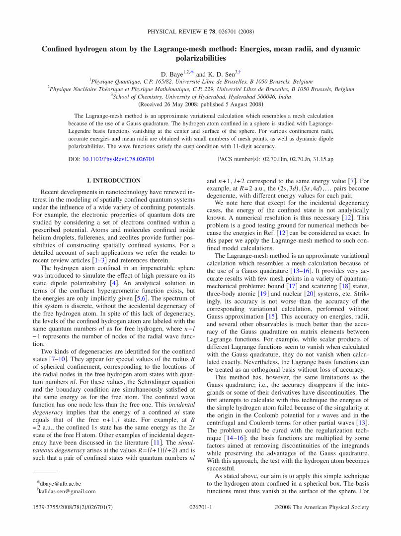
TABLE I. Convergence of energies E and mean radii of the ground state of the confined hydrogen atomfor R=2 and 10 as a function of the number N of mesh points. The last column corresponds to the cuspcondition �25�. Exact results are rounded from Ref. �12�.

N E 1 /r� r� r2� ��0� /�0�

R=2

4 −0.125061 1.53624 0.8609 0.8729 −1.9945

6 −0.1250000014 1.535161756 0.85935332 0.8748247 −1.999974

8 −0.12500000000003 1.53516170643364 0.8593531742681 0.87482539412421 −1.999999946

10 −0.12500000000001 1.53516170643331 0.85935317426677 0.87482539413417 −1.999999999939

ex. −0.12500000000000 1.53516170643330 0.85935317426677 0.87482539413417 −2

R=10

10 −0.5000016 1.0000463 1.50000626 2.99931 −1.99805

15 −0.49999926328191 1.000011692830 1.49993637881 2.99945950866 −1.99999920

20 −0.49999926328153 1.00001169282110 1.49993637877150 2.9994595088658 −1.999999999944

25 −0.49999926328148 1.00001169282098 1.49993637877163 2.9994595088663 −1.999999999996

ex. −0.49999926328153 1.00001169282108 1.49993637877151 2.9994595088658 −2

CONFINED HYDROGEN ATOM BY THE LAGRANGE-MESH… PHYSICAL REVIEW E 78, 026701 �2008�

026701-3

III. RESULTS AND DISCUSSION

A. Energies and mean radii

Equation �19� provides energies for an arbitrary potentialV. In particular, one can test the correctness of the code withV=0. From now on, we choose the Coulomb potential V=−1 /r.

With the Lagrange-mesh technique, we calculate the en-ergies of system �13� for some values of the confinementradius R. The convergence is very fast as illustrated by TableI. At R=2, the ground-state energy is exactly E=−1 /8because of the incidental degeneracy. One observes thatthe convergence is exponential: excellent results are already

obtained with only eight points. With N=10, the energy isnot improved because of rounding errors, but the wave func-tion becomes more accurate as shown by the better agree-ment with the cusp condition defined below in Eq. �25�. Byextrapolation, a 100-digit accuracy such as in Ref. �12� willbe reached with less than 50 mesh points in a multiprecisioncalculation. For R=10, the energy does not differ much fromthe free-hydrogen value −1 /2. Here also the convergence isexponential but with some delay. One observes that largerrounding errors make N=25 slightly less good than N=20.

The accuracy of the results in the following tables ischecked by comparing the results obtained with the men-tioned number N of points with results obtained with N+4and N+10 points and by only keeping stable digits. All digits

TABLE II. Energies E and average radii of the confined hydrogen atom for R=2 with N=20 mesh points:�a� present work and �b� exact results from Ref. �12�, except for the 2p state where the average radii are fromRef. �30�.

nl E 1 /r� r� r2�

1s �a� −0.1250000000000 1.5351617064333 0.8593531742668 0.8748253941342

�b� −0.12500000000000 1.53516170643330 0.85935317426677 0.87482539413417

2s �a� 3.3275091564964 1.6462701389774 1.0219789235879 1.3320904586151

�b� 3.32750915649647 1.64627013897734 1.02197892358789 1.33209045861518

3s �a� 9.3141504354036 1.8141208485472 1.0168625603981 1.3453611004185

�b� 9.31415043540360

2p �a� 1.5760187856062 0.97234328360280 1.14107908207279 1.4056651407853

�b� 1.57601878560634 0.97234328 1.405663

3p �a� 6.2690027919866 1.20705920187634 1.07290780001893 1.3855398769833

�b� 6.26900279198648

4p �a� 13.510584159771 1.36369836877412 1.04542352584587 1.3669819628524

3d �a� 3.3275091564964 0.83295185750304 1.27525204948509 1.7067631688822

�b� 3.32750915649647

4d �a� 9.3141504354037 1.03301318210024 1.14129322618607 1.4930470696061

�b� 9.31415043540360

5d �a� 17.8160934959697 1.17178541254853 1.08944558050605 1.4244486476031

�b� 17.81609349596967

TABLE III. Energies E and mean radii of the confined hydrogen atom for R=20: �a� present work withN=40 and �b� Ref. �12�; �c� comparison with free hydrogen.

nl E 1 /r� r� r2�

1s �a� −0.49999999999992 1.00000000000012 1.4999999999977 2.9999999999640

�b� −0.49999999999999 1.00000000000023 1.4999999999757 2.9999999999637

�c� −0.5 1 1.5 3

2s �a� −0.12498711431291 0.25017311811489 5.9926621769945 41.849320843821

�b� −0.12498711431292 0.25017311811490 5.9926621769942 41.849320843817

�c� −0.125 0.25 6 42

2p �a� −0.12499460664707 0.25007388596077 4.9965331340246 29.933020319372

�b� −0.12499460664708

�c� −0.125 0.25 5 30

3p �a� −0.05161141976110 0.13021802735253 10.654910283762 129.09441512402

�c� −0.05555555555555 0.11111111111111 12.5 180

D. BAYE AND K. D. SEN PHYSICAL REVIEW E 78, 026701 �2008�

026701-4

of the presented results, except the last one, are expected tobe correct.

Results obtained with N=20 at R=2 for various states aredisplayed in Table II. For s states, they are compared withthe �truncated� 100-digit results of Ref. �12�, when available.The agreement is excellent both for energies and mean radii.For d states, a comparison with the exact energies of Ref.�12� is also possible because of the simultaneous degeneracyproperty �7�, valid at R=2, End=E�n−1�s. Such a property doesnot exist for mean radii.

For p states, the agreement is also excellent for the ener-gies. However, mean radii in Ref. �12� are completely differ-ent from ours for the 2p state �not shown in the table�. Wenote here that our results agree well with those reported inTable IV of the earlier Ref. �30�, though using a less accuratemethod than in Ref. �12�. We think that the values in Ref.�12� are incorrect because, at R=20, they do not seem to tendtowards the free-hydrogen values 1 /r�=1 /n2, r�= 1

2 �3n2

− l�l+1��, and r2�= 12n2�5n2+1−3l�l+1��, while our results

have this behavior as shown in Table III. The results for theconfined atom are very close to those for the free atom aslong as the free-hydrogen density distribution is negligiblebeyond R.

The Lagrange-mesh method also provides approximatewave functions. To illustrate this point, we present in TableIV values of the l=0 radial density �r�=r−2�0�r�2 and of

its derivatives at the origin. This allows us to test the cuspcondition. The values of the radial function r−1�0�r� and ofits first derivative at the origin can be obtained from Eq. �9�with

�x−1f i�x��x=0 =�− 1�i+1

�xi3�1 − xi�

�23�

and

�x−1f i�x��x=0� =�− 1�i+1

�xi3�1 − xi�

� 1

xi− 1 − N�N + 1� . �24�

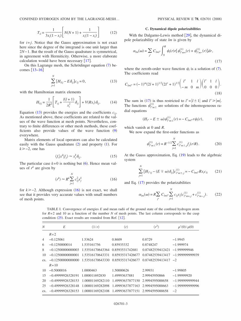
The cusp condition reads

��0��0�

= 2�r−1�0�r��r=0�

�r−1�0�r��r=0= − 2. �25�

This condition is accurately verified in Table IV. The s-statedensities at the origin are related to the corresponding ener-gies by �31�

��0��0�

=2

3�5 − 2E� . �26�

The values in Tables III and IV satisfy this relation with anaccuracy of about 10−9. Together with the cusp condition,

TABLE IV. Density and its first and second derivatives at the origin. The last column is a test of the cuspcondition and should be compared with −2.

nl �0� ��0� ��0� ��0� /�0�

R=2 �N=20�1s 9.496131945033 −18.9922638902 33.23646179 −2.000000000010

2s 20.679450381857 −41.3589007639 −22.81657942 −2.000000000010

3s 37.81519138482 −75.630382772 −343.5712035 −2.000000000060

R=20 �N=40�1s 4.0000000000000 −7.99999999993 16.000000004 −1.99999999998

2s 0.5005342706145 −1.00106854122 1.751861348 −1.99999999998

3s 0.2221433387561 −0.44428667751 0.755263078 −1.99999999998

0

0.2

0.4

0.6

0.8

1

1.2

0 2 4 6 8 10r

ψ1s

R = 2

R = 4

R = 10

x 100

R = 10 R = ∞

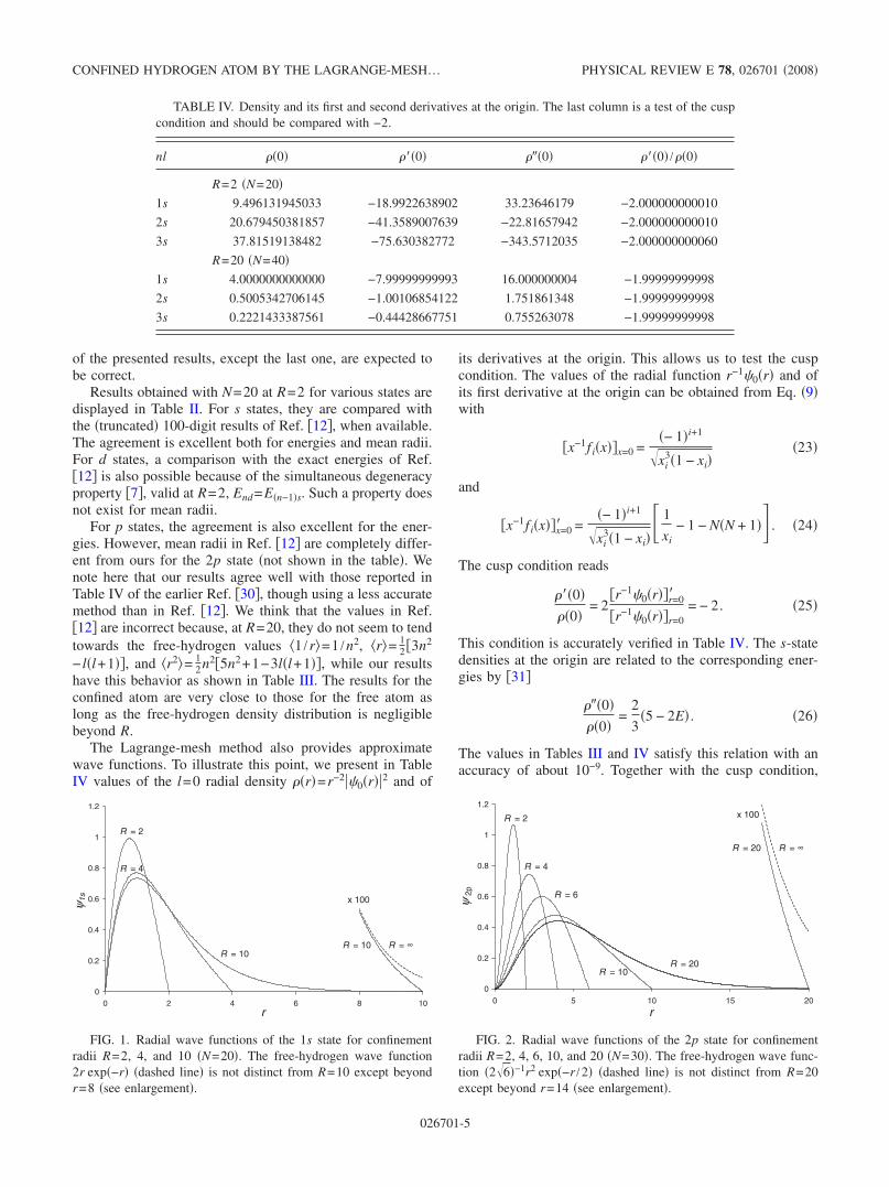
FIG. 1. Radial wave functions of the 1s state for confinementradii R=2, 4, and 10 �N=20�. The free-hydrogen wave function2r exp�−r� �dashed line� is not distinct from R=10 except beyondr=8 �see enlargement�.

0

0.2

0.4

0.6

0.8

1

1.2

0 5 10 15 20

r

ψ2p

R = 2

R = 4

R = 6

R = 10R = 20

R = 20 R = ∞

x 100

FIG. 2. Radial wave functions of the 2p state for confinementradii R=2, 4, 6, 10, and 20 �N=30�. The free-hydrogen wave func-tion �2�6�−1r2 exp�−r /2� �dashed line� is not distinct from R=20except beyond r=14 �see enlargement�.

CONFINED HYDROGEN ATOM BY THE LAGRANGE-MESH… PHYSICAL REVIEW E 78, 026701 �2008�

026701-5

this confirms the accuracy of the s wave functions near theorigin. At large R, the density at the origin and its derivativesare very close to the free-hydrogen values for the 1s state.

The wave function �1s is displayed in Fig. 1 for severalvalues of the confinement radius R. For R=10, the confinedwave function is hardly distinguishable from the free-hydrogen one. At small r values, the confined wave functionis slightly larger to ensure normalization to unity. They sharefive common digits between r=2 and r=4. Beyond r=4, theunconfined wave function is slightly larger. For r valuesaround 6, the difference is about 0.1%. At r=8, it reaches3%. Beyond this value, the two functions behave quite dif-ferently.

The wave function �2p displayed in Fig. 2 shows a similarbehavior. The R=10 confined wave function is now differentfrom the free-hydrogen one because the free-hydrogen wavefunction is still large at r=10. For R=20, the confined andunconfined wave functions are very close up to r=14 wherethe difference becomes larger than 1%.

B. Dynamic dipole polarizabilities

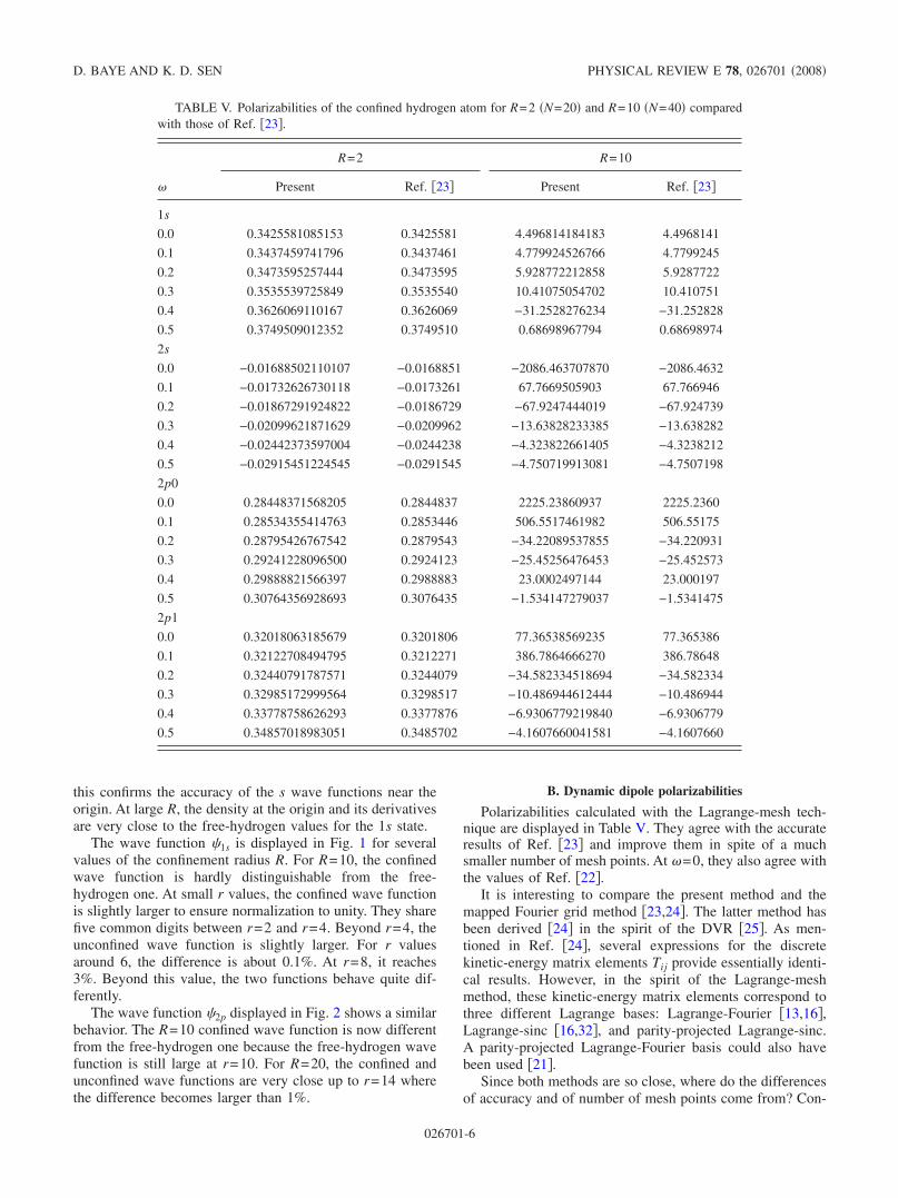
Polarizabilities calculated with the Lagrange-mesh tech-nique are displayed in Table V. They agree with the accurateresults of Ref. �23� and improve them in spite of a muchsmaller number of mesh points. At �=0, they also agree withthe values of Ref. �22�.

It is interesting to compare the present method and themapped Fourier grid method �23,24�. The latter method hasbeen derived �24� in the spirit of the DVR �25�. As men-tioned in Ref. �24�, several expressions for the discretekinetic-energy matrix elements Tij provide essentially identi-cal results. However, in the spirit of the Lagrange-meshmethod, these kinetic-energy matrix elements correspond tothree different Lagrange bases: Lagrange-Fourier �13,16�,Lagrange-sinc �16,32�, and parity-projected Lagrange-sinc.A parity-projected Lagrange-Fourier basis could also havebeen used �21�.

Since both methods are so close, where do the differencesof accuracy and of number of mesh points come from? Con-

TABLE V. Polarizabilities of the confined hydrogen atom for R=2 �N=20� and R=10 �N=40� comparedwith those of Ref. �23�.

�

R=2 R=10

Present Ref. �23� Present Ref. �23�

1s

0.0 0.3425581085153 0.3425581 4.496814184183 4.4968141

0.1 0.3437459741796 0.3437461 4.779924526766 4.7799245

0.2 0.3473595257444 0.3473595 5.928772212858 5.9287722

0.3 0.3535539725849 0.3535540 10.41075054702 10.410751

0.4 0.3626069110167 0.3626069 −31.2528276234 −31.252828

0.5 0.3749509012352 0.3749510 0.68698967794 0.68698974

2s

0.0 −0.01688502110107 −0.0168851 −2086.463707870 −2086.4632

0.1 −0.01732626730118 −0.0173261 67.7669505903 67.766946

0.2 −0.01867291924822 −0.0186729 −67.9247444019 −67.924739

0.3 −0.02099621871629 −0.0209962 −13.63828233385 −13.638282

0.4 −0.02442373597004 −0.0244238 −4.323822661405 −4.3238212

0.5 −0.02915451224545 −0.0291545 −4.750719913081 −4.7507198

2p0

0.0 0.28448371568205 0.2844837 2225.23860937 2225.2360

0.1 0.28534355414763 0.2853446 506.5517461982 506.55175

0.2 0.28795426767542 0.2879543 −34.22089537855 −34.220931

0.3 0.29241228096500 0.2924123 −25.45256476453 −25.452573

0.4 0.29888821566397 0.2988883 23.0002497144 23.000197

0.5 0.30764356928693 0.3076435 −1.534147279037 −1.5341475

2p1

0.0 0.32018063185679 0.3201806 77.36538569235 77.365386

0.1 0.32122708494795 0.3212271 386.7864666270 386.78648

0.2 0.32440791787571 0.3244079 −34.582334518694 −34.582334

0.3 0.32985172999564 0.3298517 −10.486944612444 −10.486944

0.4 0.33778758626293 0.3377876 −6.9306779219840 −6.9306779

0.5 0.34857018983051 0.3485702 −4.1607660041581 −4.1607660

D. BAYE AND K. D. SEN PHYSICAL REVIEW E 78, 026701 �2008�

026701-6

trary to the present method, the mapped Fourier grid methoddoes not regularize the singularity of the Coulomb potentialand of the centrifugal term. The accuracy of the Gauss-Fourier �16� approximation hidden in the Fourier gridmethod is restricted by this singularity and higher numbersof mesh points need be used.

IV. CONCLUSIONS

The Lagrange-mesh approximation provides very accu-rate energies and wave functions of the confined hydrogenatom with small numbers of mesh points. The high accuracyreached requires the use of a regularization of the Coulomband centrifugal singularity at the origin. This is the maindifference with the mapped Fourier grid method of Refs.�23,24� which requires many more mesh points. We did not

attempt to reach the accuracy of the 100-digit results of Ref.�12�. However, with multiprecision arithmetics, the accuracyof the Lagrange-mesh method can still become much better.

The simplicity of the method allows fast and accuratecalculations of various properties of the atom such as meanradii, densities, etc. In particular, the Lagrange-mesh methodhas been found efficient to calculate highly accurate dynami-cal polarizabilities in this simple problem. It would thus beinteresting to apply it to the calculation of polarizabilities ofthree-body atomic or molecular Coulomb systems.

ACKNOWLEDGMENTS

This text presents research results of the Belgian ProgramNo. P6/23 on interuniversity attraction poles initiated by theBelgian-state Federal Services for Scientific, Technical andCultural Affairs �FSTC�.

�1� W. Jaskolski, Phys. Rep. 271, 1 �1996�.�2� A. L. Buchachenko, J. Phys. Chem. B 105, 5839 �2001�.�3� V. K. Dolmatov, A. S. Baltenkov, J.-P. Connerade, and S. T.

Manson, Radiat. Phys. Chem. 70, 417 �2004�.�4� A. Michels, J. de Boer, and A. Bijl, Physica �Amsterdam� 4,

981 �1937�.�5� A. Sommerfeld and H. Welker, Ann. Phys. 32, 56 �1938�.�6� E. Ley-Koo and S. Rubinstein, J. Chem. Phys. 71, 351 �1979�.�7� V. I. Pupyshev and A. V. Scherbinin, Chem. Phys. Lett. 295,

217 �1998�.�8� V. I. Pupyshev and A. V. Scherbinin, Phys. Lett. A 299, 371

�2002�.�9� S. Goldman and C. Joslin, J. Phys. Chem. 96, 6021 �1992�.

�10� B. L. Burrows and M. Cohen, Phys. Rev. A 72, 032508�2005�.

�11� K. D. Sen, J. Chem. Phys. 122, 194324 �2005�.�12� N. Aquino, G. Campoy, and H. E. Montgomery, Jr., Int. J.

Quantum Chem. 107, 1548 �2007�.�13� D. Baye and P.-H. Heenen, J. Phys. A 19, 2041 �1986�.�14� M. Vincke, L. Malegat, and D. Baye, J. Phys. B 26, 811

�1993�.�15� D. Baye, M. Hesse, and M. Vincke, Phys. Rev. E 65, 026701

�2002�.�16� D. Baye, Phys. Status Solidi B 243, 1095 �2006�.�17� D. Baye, M. Vincke, and M. Hesse, J. Phys. B 41, 055005

�2008�.�18� M. Hesse, J.-M. Sparenberg, F. Van Raemdonck, and D. Baye,

Nucl. Phys. A 640, 37 �1998�.�19� M. Hesse and D. Baye, J. Phys. B 32, 5605 �1999�; 34, 1425

�2001�; 36, 139 �2003�.�20� P. Descouvemont, C. Daniel, and D. Baye, Phys. Rev. C 67,

044309 �2003�.�21� D. Baye, J. Phys. B 28, 4399 �1995�.�22� H. E. Montgomery, Jr., Chem. Phys. Lett. 352, 529 �2002�.�23� S. Cohen, S. I. Themelis, and K. D. Sen, Int. J. Quantum

Chem. 108, 351 �2008�.�24� S. Cohen and S. I. Themelis, J. Chem. Phys. 124, 134106

�2006�.�25� J. C. Light, I. P. Hamilton, and J. V. Lill, J. Chem. Phys. 82,

1400 �1985�.�26� G. Szegö, Orthogonal Polynomials �American Mathematical

Society, Providence, RI, 1967�.�27� Handbook of Mathematical Functions, edited by M.

Abramowitz and I. A. Stegun �Dover, New York, 1970�.�28� D. Baye, M. Hesse, J.-M. Sparenberg, and M. Vincke, J. Phys.

B 31, 3439 �1998�.�29� A. Dalgarno and J. T. Lewis, Proc. R. Soc. London, Ser. A

233, 70 �1955�.�30� N. Aquino, Int. J. Quantum Chem. 54, 107 �1995�.�31� Á. Nagy and K. D. Sen, J. Chem. Phys. 115, 6300 �2001�; K.

D. Sen and H. E. Montgomery, Jr., Int. J. Quantum Chem. �tobe published�.

�32� C. Schwartz, J. Math. Phys. 26, 41 �1985�.

CONFINED HYDROGEN ATOM BY THE LAGRANGE-MESH… PHYSICAL REVIEW E 78, 026701 �2008�

026701-7