Embed Size (px)
Citation preview
RAIROMODÉLISATION MATHÉMATIQUE
ET ANALYSE NUMÉRIQUE
V. BARBU
K. KUNISCH
W. RINGControl and estimation of the boundary heattransfer function in Stefan problemsRAIRO – Modélisation mathématique et analyse numérique,tome 30, no 6 (1996), p. 671-710.<http://www.numdam.org/item?id=M2AN_1996__30_6_671_0>
© AFCET, 1996, tous droits réservés.
L’accès aux archives de la revue « RAIRO – Modélisation mathématique etanalyse numérique » implique l’accord avec les conditions générales d’uti-lisation (http://www.numdam.org/legal.php). Toute utilisation commerciale ouimpression systématique est constitutive d’une infraction pénale. Toute copieou impression de ce fichier doit contenir la présente mention de copyright.
Article numérisé dans le cadre du programmeNumérisation de documents anciens mathématiques
http://www.numdam.org/
HATHEMATICAL MODELLING AND NUMERICAL ANALYSISMODÉLISATION MATHÉMATIQUE ET ANALYSE NUMÉRIQUE
(Vol. 30, n° 6, 1996, p. 671 à 710)
CONTROL AND ESTIMATION OF THE BOUNDARY HEAT TRANSFERFUNCTION IN STEFAN PROBLEMS
by V. B A R B U (*) ( ' ) , K. K U N I S C H ( Î ) (2) a n d W . R I N G (:[:) ( 3 )
Résumé. — On donne ici un procédé d'approximation pour l'identification de la fonction detransfert du problème de Stefan. Le problème à résoudre équivaut à trouver une commande detype feedback pour le contrôle de surface de solidification. Les méthodes utilisées ici sont cellesissues de l'Analyse Convexe dans les espaces de Hubert. Des résultats numériques sont donnésdans un cas particulier.
Abstract. —An approximation procedure for the identification of a nonlinear boundary heattransfer f une t ion in a o ne phase Stefan p rob le m is pre sent éd. Alternatively the p rob le m can beviewed as constructing a feedback c ont rol law for the contrat of the solidification surface in theStefan problem. The analysis is based on Hubert space methods and convex analysis techniques.N urne ri cal results combining two regularization methods are pres ent éd.AMS classification : 49A22, 32R30.
Key words : One phase Stefan problem, free moving boundary, inverse problem, feedbackcontrol, convex functions, regularization techniques.
1. INTRODUCTION
Let Q be a bounded domain in W\ n 5= 1 with a C u boundary F and let{Q{ : t e [0, 7]} be a family of monotonically increasing (strict) subdomainsof Q with the property that F is contained in the boundary of Qt for ailt G [0, 7] . To express {Qt : t e [0, 7]} analytically, the existence of a func-tion a : QT —> [0, 7] is assumed with the properties that a e C2(QT\QQ),\Va(x)\ ^ 0 for ail xe ~QT\QQy a(x) = 0 on ö 0 and such that
QT\ a(x) for 0
(*) Research partially supported by NSF Grant DMS-91-11794.( î ) Research partially supported by Christian Doppler Laboratory for Parameter Identifica-
tion and Inverse Problems.(:10 Research partially supported by Spezîalforschungsbereich Optimierung und Kontrolle.(') Institute of Mathematics University of lasi, RO-6600 Iasi, Romania.(2) Fachbereich Mathematik Technische Universitat Berlin D-10623 Berlin, Germany.(3) Institut für Mathematik Technische Universitat Graz A-8010 Graz, Austria.
M2 AN Modélisation mathématique et Analyse numérique 0764-583X/96/06/S 7.00Mathematical Modelling and Numerical Analysis (Ç) AFCET Gauthier-Villars
672 V. BARBU, K. KUNISCH, W. RING
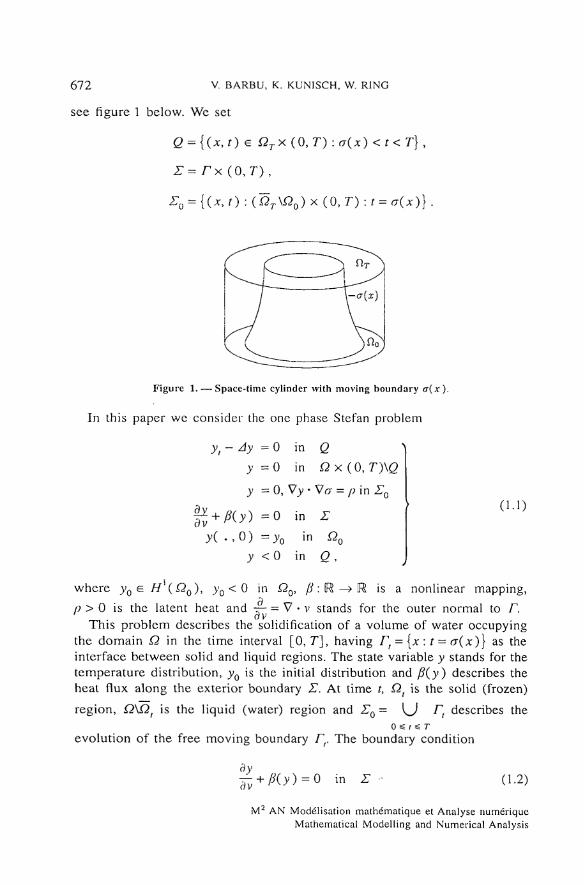
see figure 1 below. We set
G = { ( J C , 0 G QTx ( 0 , 7 ) :a(x) < t < 7} ,
Z= Fx ( 0 , 7 ) ,
Figure 1. — Space-time cylinder with moving boundary a(x).
In this paper we consider the one phase Stefan problem
yt - Ay = 0 in Q
y - 0 in Qx (OtT)\Q
y = 0, Vy • Va = /; in EQ
fï + #30 =0 in 27y( . , 0) = yQ in Qo
y < 0 in g ,
(1.1)
where y0 < 0 in3
/? : is a nonlinear mapping,
/> > 0 is the latent heat and — = V • v stands for the outer normal to F.This problem describes the solidification of a volume of water occupying
the domain Q in the time interval [0,7] , having Ft = {x : t - cr(x)} as theinterface between solid and liquid régions. The state variable y stands for thetempérature distribution, yQ is the initial distribution and fi(y) describes theheat flux along the exterior boundary 27. At time t, Qt is the solid (frozen)
région, Q\Qf is the liquid (water) région and ZQ = \^J Ft describes the
évolution of the free moving boundary Fr The boundary condition
in (1.2)
M2 AN Modélisation mathématique et Analyse numériqueMathematical Modelling and Numerical Analysis
CONTROL OF STEFAN PROBLEMS 673
describes a possibly nonlinear boundary heat transfer law. In the linear casewith /?(>') =Ay> fi > 0, one refers to (1.2) as radiation condition. If /?,together with /; and >'o are given, then the direct Stefan problem consists indetermining the température distribution y together with the free boundaryEQ which is characterized by a from (1.1).
Here we shall consider the following inverse problem : Given the functiona détermine ft from a class of admissible functions, such thatEQ = {(x, r) : t = (j(x) = a ( / i ; x)} is the free boundary of the resultingone phase Stefan problem. This problem can be thought of in two differentways. First it constitutes the inverse problem of identifying the unknownboundary heat transfer coefficient from overspecifled boundary data on EQ.Secondly it describes a feedback control problem for the one phase Stefanproblem with boundary control :
3yóv
and with the control u in the feedback form :
3yT" = » i n % (1-3)
(1.4)
The objective is to steer the free boundary a = rr(/i) to some a priori desircdsolidification surface. We refer to [HN, HS] tbr results and références relatedto the control of Stefan problems.
The class of admissible heat transfer functions (or feedback control laws) ischosen to be
sé = {/?= dj: with y : U -> R convex, continuous,7'(0 ) = 0, 0 e //(O)
and a0 + a>0 r2 ^ j(r) ^ a, + œl r2 for all r e IR},
where 0 < coQ< col9 and a0 < a{ are constants and dj, inapping M. into theset of all subsets of R, is the subdifferential of ƒ Thus, fi is a monotone graphand the boundary condition on E has to be replaced by
P() (1 .5)
The above inverse problem will be formulated as least squares problem :
minimize ( Vy • Vrr — /; y dx dt•U» \ (1.6)
subject to/? e sé and y e ƒƒ'( Q) satisfying
vol. 30, n° 6, 1996
674 V. BARBU, K. KUNISCH, W. RING
yt~Ay = 0 in Q )y = 0 in EQ
^ + Piy) 3 0 in ^ ( L 7 )
y{ . , 0 ) =3>0 in
We note that the solution 3? of (1.7) is not effected by replacing j byj + constant. This motivâtes the constraint j(0) = 0 in the définition ofse'. One of the main goals of this paper is the analysis of (1.6) by convexanalysis techniques. In particular, the nonlinear boundary condition will besimplified by a substitution similar to operator splitting or the mixed üniteelement method. Numerically the solution of the inverse problem of identi-fying the heat transfer coefficient on one part of the boundary from measure-ments on other parts is related to the sideways heat équation [C] which is anotoriously illposed problem. The second goal of this paper is therefore thedescription of a numerical algorithm for the identification of the boundary heattransfer coefficient (or the feedback control law) /? in (1.1), which proved tobe successful on a series of test examples.
The plan of the paper is the following one. In Section 2 we shall studywell-posedness of the closcd loop System (1.7) in a Hubert space Framework.Section 3 is devoted to proving existence and convergence of suboptimalsolutions to (1.6). An approximation process of similar kind was already usedin [BK1, BK2] for the identification of nonlinear elliptic and parabolicboundary value problems. Roughly speaking the nonlinear boundary conditionin (1.7) is decoupled via (1.3), (1.4), resulting in a parabolic optimal controlproblem on the non-cylindrical domain Q in the control variables v and j . InSection 4 a maximum principle type resuit for this problem is given. Numeri-cal algorithms and tests are presented in Section 5.
We shall use standard notation for the spaces of square integrable functionsand Sobolev spaces on Qt, Q and E, Given a îower semicontinuous functioncp from a Hubert space X to [R = (-<», 00] we shall dénote by 'àtp itssubdiffercntial, i.e. :
c)(p(x) - {w e X : (p(x) ^ <p( 11) + (coy x - u) for all u e X) ,
and by
(p* : X —> f8 its conjugate function defined by ,
<P*(p) = SUP {(p, u) — <p(u) : u e X} , forp e X,
where ( • , . ) dénotes the scalar product on X. We refer to [BI] for furtherresults from convex analysis which will be used in this paper.
M2 AN Modélisation mathématique et Analyse numériqueMathematica! Modelling and Numerical Analysis
CONTROL OF STEFAN PROBLEMS
2. THE NONLINEAR CLOSED LOOP SYSTEM
675
We shall study here the nonlinear system (1.7) which we repeat forconvenience :
yt - Ay = 0 in Q ^
y = 0 in r 0
in
y ( x , 0 ) = yo(x) in QQ .
Here fi is a maximal monotone graph in IR x IR such that
and 0
This implies that /? = öy, where y :function such that
is a convex and continuous
= i n f { / ( r ) : r
see [BI], p. 71. We shall call y a (variational) solution of the boundary valueproblem (2.1), if it is an element of
such that
f (-JQ
daxdt
f y(x, TXy(x,T)-zUT))dx
(2.2)
for all z e V.lt is simple to check that every classical solution to (2.1) satisfies(2.2). Moreover we have the following result :
vol. 30, nQ 6, 1996
676 V. BARBU, K. KUNISCH, W. RING
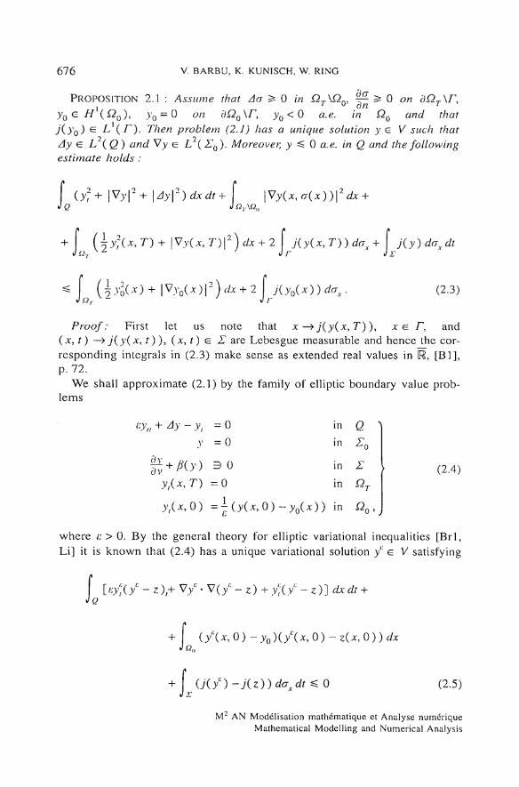
PROPOSITION 2.1 : Assume that Aa S= 0 in QT\Qnt ^ S* 0 on öQT\F,' v fin r
v0 e ƒƒ ( y0 = 0 on dQQ \F, yQ < 0 a.e. in QQ and thaï
j(y0) e L (F). Then problem (2J) lias a unique solution y e V such thatAy e L"(Q) and Vy e L (^ 0 ) . Moreover, y 0 a.e. m 2 and the followingestimate holds :
|V>-|2+ |zJ>|2)dxdt+ \ \Vy(x,<7(x))\2dx +JnT\a„
y ' U 7-) + \Vy(x, T)\2)dx + 2 j KyU T))dax
( 2 V° ( -V } + I V y o ( ^ ) 12 ) + 2 J y ( Vo(
dax dt
dax . (2-3)
Proof: First let us note that x —*j(y(x, T)), x e F, and(x, r) —> j'(y(x, t) ), (x, r) e E are Lebesgue measurable and hence the cor-responding intégrais in (2.3) make sense as extended real values in R, [Bl],p. 72.
We shall approximate (2.1) by the family of elliptic boundary value prob-lems
% + Ay -yt = 0
V = 0
U + /?(>') 3 0
in Q
in Eo
in E
in Q7
in Dn
(2.4)
where /; > 0. By the gênerai theory for elliptic variational inequalities [Brl,Li] it is known that (2.4) has a unique variational solution ƒ e V satisfying
/ • V( ƒ - ƒ -
+ f~j(z))daxdt ^ 0 (2.5)
M2 AN Modélisation mathématique et Analyse numériqueMathematical Modelling and Numerical Analysis
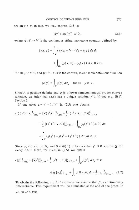
CONTROL OF STEFAN PROBLEMS 677
for all z e V. In f act, we may express (2.5) as
Ayc+dy/(/) ^ 0, (2.6)
where A : V —» Vis the continuous affine, monotone operator defined by
dt( Ay, z ) = ( sy zt + VyVz + ytzJQ
+ f (y(xt0)-yQ(x))zU0)dx
for all yy z e K, and y/ : V —> [R is the convex, lower semicontinuous function
W(y) ~ j(y)dox for all j e V.J r
Since A is positive definite and y/ is a lower semicontinuous, proper convexfunction, we infer that (2,6) has a unique solution / G V, see e.g. [Bl],Section 3.
If one takes z = ƒ' — (yc)+ in (2.5) one obtains
fSince yQ < 0 a.e. on i20 and 0 e c[/(0) it follows that yc ^ 0 a.e. on Q forevery e > 0. Next, for z = 0 in (2.5) we obtain
«rx A = i bol^ 0 u ) • (2.7)
To obtain the following a priori estimâtes we assume that fi is continuouslydifferentiable. This requirement will be eliminated at the end of the proof. In
vol. 30, n° 6, 1996
678 V. BARBU, K. KUNISCH, W. RING
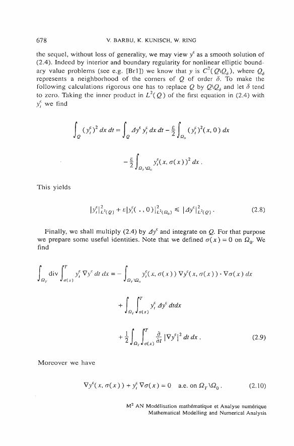
the sequel, without loss of generality, we may view yc as a smooth solution of(2.4). Indeed by interior and boundary regularity for nonlinear elliptic bound-ary value problems (see e.g. [Brl]) we know that y is C2(Q\QÔ), where Qô
represents a neighborhood of the corners of Q of order ö. To make thefollowing calculations rigorous one has to replace Q by Q\QÓ and let S tendto zero. Taking the inner product in L2(Q) of the first équation in (2.4) withyi:
t we find
(/t)\xi0)dx
U)fdx.
This yields
0o)^ W\l\Q)- (2-8)
Finally, wc shall multiply (2.4) by AyL and integrate on Q. For that purposewe prépare some useful identities. Note that we defined rr(x) = 0 on QQ. Wefind
f div f /tVyEdtcU = - f y;(x,a(x)) Vy(x,a(x))-Va(x) dxJ Q, J a(.v) J Qr\Q{i
r+ I y'Aydtdx
I QTJo(x)
2 f r à^ JarJ<j(x) öl
Moreover we have
- 0 a.e. on;Q7,YQ0. (2.10)
M2 AN Modélisation mathématique et Analyse numériqueMathematical Modelling and Numerical Analysis
CONTROL OF STEFAN PROBLEMS 679
Combining (2.9), (2.10) and using the divergence theorem we obtain
f yt Ay dxdt=\ div f y] V / dt dx
+ f y-{x, a{x)) V/(x, <T(x) ) Va(x) dx
-4 f
= f r^V/.v^^v- f |V/(x,a
QT\Q0
|V/(x,0)|2</x
= f Ü(yeU0)-KyeUT)))]d<Jx-±f |V/(x,a(x))|2^x
-\ \ |v/(x,r)|2r/x + j f |vy;(x,o)|2^xs (
where in the last step we used the boundary condition on E.Similarily we find for a.e. x e QT
f y£ttA/dt = -/tUfT(x))A/(x,a(x))-d[v f y; V^
JITU) Jff(jf)
vol. 30, n° 6, 1996
680 V. BARBU, K. KUNISCH, W. RING
and upon integrating this equality on QT
f /t(A/dt = - f /t(xya(x))dxvx(V/(x,<j(x)))dxJQ Jaf\Qti
- f yct(x, 0)Ay\x,0)dx
Due to the boundary condition on 27 and the initial condition for yct we obtain
/„ A/ dxdt = - \ /,( x,a(x)) divx( V/( x,(j(x)))dxQ
<>«o
.v*|2rfrrf/ + l^jLfiifïd^dt. (2.12)
where we use the temporary assumption that fi is continuously differentiable.Combining (2.4), (2.11) and (2.12) implies that
| Ây \2dxdt= y* Ay dx di - s ytt Ay dx dtJQ J Q J Q
\Vy\x,0)\2dx
- i f \Vy\x,G{x))\2dxz JiiT\a„
- j Ky'U T) ) dax +1 K/U 0) ) dox
M2 AN Modéiisaiion mathématique et Analyse numériqueMathematical Modelling and Numerical Analysis
CONTROL OF STEFAN PROBLEMS 681
+ f fi(yEU0)Xyo(x)-y\xt0))daxir
(2.13)
Here we use the assumption that >0U« ( ,\r=^- L e t u s n o t e t h a t
and by (2.10)
= f ( ^ i f
vol. 30, n° 6, 1996
682 V. BARBU, K. KUNÎSCH, W. RING
whcre n dénotes the outer normal to QT\QQ. In the last estimate we used
>/:(x, 0) = 7 ( / ( x> 0) - yQ{ x )) = 0 a.e. on dQQ\F and the assumption that
Âa ^ 0 a.e. on QT\QQ and -y- 0 on düT\F. Using these estimâtes in(2.13) one obtains
f \Vyc\2dxdt + \
\ \V/f\2dxdt + ±l |V(/(x, 0) - yo(x))\2dx
x))dax. (2.14)r
Combining (2.7), (2.8) and (2.14) we find
2 ƒ y( / (^ n ) v + J ^(/) dcjxdt
2 o (2-15)
By estimate (2.15) it follows that there exists J G V with yt andAy e L {Q) such that on a subsequence of yc we have
ƒ —> y weakly in Hl(Q), strongiy in L2(Q) ,
^ ™> J f weakly in L2(Q) ,
Jy^ —> / l ^ weakly in L 2 (Q) ,
e^ -> 0 stronglyin L 2 (Ö) , (2.I6)
/ (x , 0) -> ><x, 0) stronglyin L2(I30),
y —-» j stronglyin L2{£) ,
V / -> Vj; weakly in L2(2-Q) , as e -> 0 + .
M2 AN Modélisation mathématique et Analyse numériqueMathematical Modeliing and Numerical Analysis
CONTROL OF STEFAN PROBLEMS 683
In particular we infer that the trave of Vy on Eo is well-defined in the senseof Vy e L2{E0). Letting i: tend to zero in (2.5) we find that y is a solution to(2.1) which satisfies the estimate (2.3). Since yr ^ 0 a.e. in Q for allt: > 0 we deduce that y ^ 0 a.e. in Q.
To eliminate the regularity requirement on ƒ? that we made before (2.8) oneapproximates ƒ? by a family of continuously differentiable, monotonicallyincreasing functions px : R —> IR with P*(0) = 0, which satisfy in addition
jX(i) lim inf jX(r;) 5= j(r) whenever rx-ï r in
(ii) lim j\r)=j(r) for all r e IR,
(iii) | / / ( r ) - px(r)\ ^C for a constant C independent of X > 0,r e R,
where
j\r)=\ fT\s)ds and p} = X~ \ 1 - ( Î + Ajff)" ' )Jo
A spécifie choice for such a family of functions is given by
=J -
For details we refer to [BI], pp. 157, 171, 322. Repeating the abovearguments with P replaced by pA one obtains a double indexed family ofvariational solutions yCl/ to (2.4) with ƒ? replaced by px satisfying
• 1+ f ( / ' U 0) -y 0 ) (/%A(x, 0) - z(x, 0) )
iI ^ ^ 0 . (2.17)
vol. 30, n° 6, 1996
684 V. BARBU, K. KUNISCH, W. RING
Moreover the following a priori estimate holds :
f ( (yïX f+\ Vƒ• î 2 + | V/- } f )dxdt+\ | V ƒ •'(x,<r(x))\2dx
2 ƒ ƒ (ƒ ' \x, 7) ) + ƒ ƒ ( ƒ 'A ) daxdt
(2.18)
Now let us fix e > 0. Due to (2.18) there exists ƒ e HX{Q) with y* andAy' e L2(Q) and a subsequence of {/tA};,>o t n a t converges as X —> 0 + toy in the sensé of (2.16) with e — 0 + replaced by X —> 0 + . Moreover thereexist functions d G L2(F) and <J2 e L2(E) such that
l i m / ( / ' ; X . , 7 ) ) ->£ , weaklyin L2( T) (2.19)
•À/ /:, /lim / ( / l X ) -> £2 weakly in L ' ( ^ ) (2.20)
Due to (iii) we have
|/O)| ^ U;(r)| + clrl fora11
and hence using Fatou's lemma for the term j (y€< ) da dt and Lebesgue's\ j (y ,
bounded convergence theorem for f\z) daxdt we can pass to the limit as
X -» 0+ in (2.17) and (2.18). In this way we obtain (2.5) and (2.15) for everys > 0. Passing to the limit with respect to c —> 0 we obtain existence of asolution to (2.1) which satisfies the estimate (2.3) for every ƒ? satisfying thecondition specified at the beginning of this section.
M2 AN Modélisation mathématique et Analyse numériqueMathematical Modeliing and Numerical Analysîs
CONTROL OF STEFAN PROBLEMS 685
The uniqueness of y is immédiate by the variational formulation (2.2). Thiscomplètes the proof.
3. A LEAST SQUARES APPROACH TO IDENTIFY THE BOUNDARY HEAT TRANSFERFUNCTION
We shall consider the optimization problem
minimize ( Vj • Va - /; )2 dax dt
subject to/? e sS and toy e H{(Q) a solution to (2.1 ) .(P)
Throughout this section we assume that yQ and a satisfy the assumptions ofProposition 2.1. Then ( P ) is well-defined as a conséquence of (2.3).
THEOREM 3.1 : Problem (P) lias at least ane solution(y*,/?*) e Hl(Q)x sf.
Proof, Let d dénote the infimum in problem (P) andlet {(yn>Pn)} c Hl{Q) x J / be a minimizing séquence satisfying
(3.1)
with yn the variational solution to
fyn =0 ini70
0(3.2)
Due to (2.3) and the properties of éléments in sé there exists a constant C suchthat
for all n.It follows that there exists y e Hl(Q) with zfv e L2( 2 ) such that for a
subsequence
yn ~^ y w e a^ly in Hl ( Q ) and
vol, 30, n° 6, 1996
Vy weakly in L2( EQ ) .
686 V. BARBU, K. KUNISCH, W. RING
Taking lim inf in (3.1) we infer that d = | Vy • Va - p\2jj{Li)y It remains topass to the limit in
f (->'„(>•„ - z), + V.y„ • V(>-, -z))clxdt+ f (/,(ƒ„) -JM))d<rxdt
+ f ynUTXyH(x9T)-z(x,T))dx
~ f yö(x)(yn(xJÖ)-z(x,0))dx^0
for all z e V- This is simple for ail terms except for the second. To take thelim inf on that term one uses the Arzela-Ascoli theorem to conclude conver-gence of {jn} in C(I) for every compact lezR, By Fatou's lemma andLebesgue's bounded convergence theorem (using jn e Jf ) we obtain
j{ y ) dax dt + j(z) daK dt ^ lim inf jn(yn ) dax dt
+ lim inf jn(z) daxdt,
and the desired resuit follows.Next we approximate problem (P) by the following family of optimal
control problcms in the control variable v :
minimize < ( Vy • Vrr — /; )" daK dt +
i f «>:subject toy e H\Q)J e Jf\ v e L2(Z)and >' a variational solution to
yf - Ay = 0 in Q |
y = 0 in i7n
in(3.4)
vUO) =yo(x) inr20,
M2 AN Modélisation mathématique et Analyse numériqueMathematical Modelling and Numerical Analysis
CONTROL OF STEFAN PROBLEMS 687
where A > 0, and
X = {j : R -» R is convex, continuous,y(0 ) = 0, 0 G dy'(O), (3.5)
a0 + a;0 r2 y ( O ^ a i + w, r2, for all r e IR} .
Note that sé = {/J = d/ : j e J f } .The introduction of the second term in the payofï oï ( P} ) is suggested by
the équivalence between
0 and K
at all points (x, t) E i7 where these équations are well-defined. Moreover
whenever this expression is defined. Upon setting t; = — and integrating (3.6)on E we obtain
with equality holding if and only if
y*( -^ ) + = öa.e. inZ\ (3.7)
Thus the second term in the payoff of ( P ; ) is a penalty term realizing (3.7)and (Pk) constitutes a splitting or mixed finite element method with respect
to the variable -^ for problem ( P ) .Before going further, some comments concerning (3.4) are in order. For
y0 e Hl(Q0) with yo = O a.e. in dQ0\r, and if vte L 2 ( T ) , then (3.4) hasa unique variational solution y satisfying
y(x,T)z(xyT)dx =fJ
vzdaxdt+ yo(x)z(x,Ö)dxy (3.8)r J Q()
for all {z e H\Q) : z = 0 in Zo] and
jy = 0a.e. in EO. (3.9)
vol. 30, n° 6, 1996
V. BARBU, K. KUNISCH, W. RING
Moreover y satisfies y e Hl(Q) with Ay e L2(Q) and V>-• Va e L2(270).The proof follows from the proof of Proposition 2.1, see also [B2]. It is simpleto argue that
f \Vy\2dxdt+\ y2(x,t)dx^ Cl \ y2ödx+\ v2 daxdt\ , (3.10)
Ja Ja, \ JÖ„ Jr /'e
with C independent of y0, v and t e [0, X].For gênerai f e L~(£) it follows by density arguments based on (3.10) that
(3.4) admits an unique variational solution satisfying (3.8) and (3.10) as well.
Since y{t) e Hl(Qt) for a.e. te [0, X] and \y( . , t)\2H>,Q ) dt < °°, the
Jo -, 'trace of y( t ) on #£?, is well-defined and belongs to L"( c> 2r ) for a.e.f e (0, X), so that (3.9) makes sense. In the neighborhood of 27O the solutiony of (3.4) is in fact more regular. For that purpose we introducé the domainQ'ŒQ0 (and hence Q'c:Q{ for all f e [0, X] ) with the property thatd.Q'consists of two connected components, one of which coïncides with /"andthe other lies in the interior of Qo. Then it is straightforward to argue, e.g. bya Galerkin procedure, that the solution of (3.4) satisfies in addition to (3.10)
with C independent of\y0 s HX(Q) and v e L2(£). In particular the payoffin ( P ; ) is well-defined for v e L2(Z).
We shall say that (yx,jx>v^ converges in (L2(Q))w x X x
(L2(Z))w to (yJyV), if yk-*y weakîy in L2(Q)y vÀ~^v weakly inL"(i7) and j - —>y uniformly on compact subsets of R.
THEO REM 3.2 : For every A > 0 there exists at least one solution(>'„yA,ü,)e L2(Q)x J f x L 2 ( I ) of (Px). Moreover {yÀJx,vx}.>0
contains a clusterpoint in ( L2( Q ) )w x JT x (L"( iT) )w, r/7e ƒ m ?wocomponents of every such clusterpoint are a solution of (P) andlim inf Px = \nfP.
Proof: Let (ynjn, vn) be a minimizing séquence for (/^) satisfying
(3.12)
M2 AN Modélisation mathématique et Analyse numériqueMathematical Modelling and Numerical Analysis
CONTROL OF STEFAN PROBLEMS 689
for every n G M, where yn, vn satisfy (3.4), jn e Jf and dx = inf (PA) . Due* f
to the properties of Ctif using (3.8) to eliminate the term vnyndaxdt it
follows that
for a constant C independent of n. From (3.11) it follows that { | | ( }
î & [0, T] }~= j is bounded as weîî. Consequently there exist y-; e L ( 2 ) withVyA E L 2 ( g ) and VyA • V<r e L 2 ( i7 0 ) , and i^ € L 2 ( T ) , such that on a sub-sequence, again denoted by {n}, we have
weakly in L ( Q )
weakly in L2(Q)
stronglyin L 2 ( T 0 )
weakly in L 2 ( i 7 ) .
Sinee j H e JT for ail n there exists a constant Cl independent of n such that
\ajl(r)\ + \djn(r)\^C{(\r\2+\) for ail r e U .
Consequently by the Àrzela Ascoli theorem there exists jÀ € Jf* such that
.ƒ„('") ~-*J*A(r) a n d y*,(r) - * i l ( r ) uniformly in ron
compact subsets of ER . (3.13)
It is simple to argue that (>';, v;) is a variationaî solution of (3.4), Le, that (3.8)is satisüed.
We next argue that {yoyn}~lssi is compact in L2(£). Hère yQ dénotes thetrace of y on 27. Let Hl
m(Q') = {<p e H\Q') : <p\BQ'\r= 0}. Using the factthat {PH} is bounded in L2{£) it is simple to argue that {yn} is bounded inL 2 ( (0 5 T) ;Hl(Q')) and {(>>„),} is bounded in L 2 ( (0 , 7 ) ; ' / / ' / G ' ) * ) . Forevery £ e (0, 1/2) one has the continuous injections
Hl(O') cz Hm + a(Qf) c / /^( f i ' )* .
vol. 30, n° 6, 1996
690 V. BARBU, K. KUNISCH, W. RING
with the first one being also compact. By Aubin's compactness theorem itfollows that {yn} is precompact in L2((0, T) ; Hm + \Qf) ) and hence{yoyn} is precompact in L2(£). Hence for a subsequence, again denoted bythe same symbol, we have
rQ yn -* o y>, strongly in L2{ E) . (3.14)
Since j n e J f it follows that jn(yn) ^ otQ a e - an<^ n e n c e by Fatou's lemma
and (3.13), (3.14) we fînd
îiminf f jn{yn)daxdî^ \ J;(y}) daxdt. (3.15)
Since vn —> i;; only weakly in L2(iT), taking the Iiminf inf fH(- vn) daxdt is more delicate. Based on (3.13) one can argue as in the
proof of Theorem 2.1 of [BK1] to obtain
lim inf f fn(-vn)daxdt^ \ j\(-vx) d(Txdt. (3.16)
We also have
lim I yavndrrxdt = j ykvxd(jxdt. (3.17)
Combining (3.12) and (3.15)-(3.17) we find
- f ( V V - ; 2 <x + i f ' O •* - t ?
and hence (yÀJÀ, vx) is a solution to (PA).We turn to the asymptotic behavior of ( P ; ) as  - ^ 0 + . For every
 > 0 we have
xdt
( V / V T - / ; ) 2 J(7x dt = inf P , (3.18)
where (y , j ; , v ) is any solution to (P) .
M2 AN Modélisation mathématique et Analyse numériqueMathematical Modelling and Numerical Analysis
CONTROL OF STEFAN PROBLEMS 691
Arguing as above, with (y^j^v^) replacing (ynjn, vn) we find that{\yx\tHQ)}> {|v^L2(ö)}«^I^Ufl |\ö') :fe tO,r]}, and { K | ^ m } arebounded uniformly for A > 0. Consequently there exist y e. L (Q) withV>' e L2(Q) and Vy • Va e L2(270X and v e L 2 ( i 7 ) such that on a subse-quence {Xn} of {Aj A > 0 , with lim Àn — 0 we have
y A -> y weakly in L 2( Q )V^ ( 1 -> V ^ weakly in L2( Ö )
V 3 V V c r - ^ V ^ - V a stronglyin L2(i70)
v} —> i; weakly in L2(Z) ,
as « —> oo. Moreover there exists j e ^ such that
jÀii(r) —>y(r) a n d 7 * ( ( r ) —>j*(r) uniformly in r on compact subsets of f8 .
As above one argues that
lim inf (j;(l i m i n f (j;(yx)+jl(-v )+y v )daxdt
J ry y ) + / ( - y ) + yy)<for<fr2* o ,
and by (3.18)
y(.y) + ƒ ( - ü ) + )W = 0 a.e. in E .
It follows that
v e /?(;;) a.e. in E .
Clearly (y,v) is a variational solution of (3.4) and hence (y,j,v) is avariational solution of (2.1). Moreover from (3.18)
f (VyVa-p)2d(JKdt ^ \ (Vy° . Vrr - pf daxdt ,
and thus (3 ,7, u ) is a solution to ( P ). By (3.18) it follows thatlim inf P} = inf P. This ends the proof.
x->0 +
vol. 30, n° 6, 1996
692 V. BARBU, K. KUNISCH, W. RING
In thc final rcsult of this section we return to thc control thcory interpré-tation of (P)* We shall assert that the feedback control law
u e - àjk(y) m E
with j ; the second component of the solution (y},jÀ, vx ) of ( P}) applied to theoriginal problem (P) gives a suboptimal approximating solution for thatproblem.
THEOREM 3.3 ; Let (yÀJ}) e L2(Q) x Jf be given by Theorem 3.2 andlet yx be the solution to (2.1) with fi~ djÀ. Then
y A ~ y x "^ ° cmd V ( y\ ~ yx ) -* ° strongly in L2( Q ) as k -> 0 + . (3.19)
Moreover, every subsequence {(}'; , j ; )} of {(y^j; )};t>o contains a clusterpoint (y\f) in (L2( Q) ) w X $C, which is a solution to (P) .
Proof : For every o O we have
fQ
andf f
( ( yk ), w + Vv; • Vw )dx dt - v; w dax dt = 0JQ ' J r
for ail z, vv G K Setting z = yA, w = _yA - j ^ and subtracting the aboveequality from the inequality we find
* - yÀ)\2dxdt +
+ f [/,(>I ) - hi yk ) + vk(.y* - yA )] daK dt < 0 . (3.20)
We recall from (3.18) that
)+yxvx)<toxdt**C/. f o r a l l A > 0
M2 AN Modélisation mathématique et Analyse numériqueMathematical Modelling and Numerical Analysis
CONTROL OF STEFAN PROBLEMS 693
and hence
Uiiy\) -7;.(>';.) + üx(.vl - >';.) ) dcJ,-dt ^
^ CA - f (v, y \ + j?{y) )+_,-•(_ Ü. ) ) rfCTjr rfï <= Ck .v £
Inserting this estimate into (3.20) the validity of (3.19) follows. For any
séquence {(y^^Jx,)} t n e séquence {(yxJx>vx,)} contains, due to Theo-rem 3.2, a convergent subsequence, the limit of which has the property that itsfirst two components are a solution to ( P ) .
4 . S O L V I N G P R O B L E M S (P})
Besides the obvious fact that the problems ( P ; ) are infinité dimensional andthat numericaï realization requires discretization, these problems representsome serious structural difficulties. In this section we shall address theproblems related to the numericaï treatment of the set JCthe éléments of whichare defined over an unbounded domain and are required to be strictly convex.Moreover we characterize the gradient of the cost with respect to (y,j\ v).These considérations are independent of the spatial dimension. In the follow-ing section we describe a spécifie numericaï realization in spatial dimensionone. There we shall also take into considération the inherent illposedness ofthe optimization problems : In fact, the cost functional in ( P ; ) is not coercivewith respect to v or j .
Throughout this section we shall assume that yQ e H\QO) n C(QQ), thaty0 < 0 in Qo and that y0 = 0 on öQQ\F. Then for any fJ e sé the solutiony to (2.1) satisfies
-a :=inf>0 ^ y(x, t) ^ 0 in Q (4.1)
and
- a ^ y(x,t) ^ 0 on E . (4.2)
This follows from the strong maximum principle for paraboHc équations (seee.g. [PW]), since the extrema of y in Q are not attained on E. Since in viewof (2.1) only the values of y on the range of y contribute to the value of thecost functional in ( P ) , it therefore suffices to restrict the domain of j to[—a, 0 ] . Concerning the actual problem formulation on a bounded domaintwo conflicting issues arise. On the one hand one would like to enlarge the
vol. 30, n° 6, 1996
694 V. BARBU, K. KUNISCH, W. RING
domain for y beyond [— a, 0] so that perturbed problemsw (e.g. (P;)) stillhave the property that their solutions are not effected by restricting the domainand on the other hand, enlarging the domain introduces some indeterminancyinto the problem (with adverse numerical conséquences), since the limitproblem is not effected by the values of j on the complement of [— a, 0 ] . Forthe purpose of the present section we shall restrict the domain of j to/ = [—a — C, «] for some i: ^ 0.
Another practical issue consists in the numerical realization of the convexityassumption involved in the définition of sé. This will be accomplished by anadditional regularity assumption for ƒ For computational purposes we shalltherefore consider
minimize (Vjy*Va —/;) daKdt
on (yj) e H\Q) X X \ subject to (2.1 ) with /i = dj
( ƒ > ' )
where
J T 1 ={j e H2{I) :y(0) = / ( 0 ) = O, 2 co0 *k j"(r) ^ 2w,,fora.e .re /} .
Accordingly {P}) is replaced by
minimize | ( Vy • Va - /; )
1
on(yj,v) e Hl{Q) X JT X L2{E) subject to ( 3.4).
In (P\) it is understood thditj(y) = ~ for y <£ I and j * : M i s d e f i n e dby
j\p) = sup {py-j(y) :ye 1} , for p G R .
^ ^|^(2:) m (^;) n a s D e e n added for numericalThe regularization term ^ |^ |^ ( 2 :) m ( ^purposes.
Since J^ 1 is a closed convex subset of
j = {j : / —» [R,y convex and continuous,j(0) = 0, 0 e 3 / ( 0 ) ,
a0 + a;0 r2' ( ^ ) ^ a i + cox r
2 , f o r a l l rel},
M2 AN Modélisation mathématique et Analyse numériqueMathematical Modelling and Numerical Analysis
CONTROL OF STEFAN PROBLEMS 695
and, as seen above, problem (P) can be restricted to JfTv Theorems 3.1, 3.2,and 3.3 remain valid for ( P 1 ) and (P\).
We next characterize the gradients of (P\) with respect to j and (y, v ). Atthe same time we note that (P\) can be decomposed into two convexoptimization problems. These are :
1) For flxed j e JT1 solve the optimal control problem
minimize (Vy • Va - p)2 daxdt + \V\L\E) +
/ ( - v) + yv) daxdt (4.3)
2(on (y,v) e ƒƒ'( Q) x L2( 27) subject to (3.4) .
2) For fixed (y,v)e HX(Q) x L2(Z) solve the minimization problem
minimize (j(y) + J: ( - ^ ) ) daxdt
subject to ; e J5T1 . (4.4)
We turn to the characterization of the gradients of the cost functionals in (4.3)and (4.4). Problem (4.3) is a convex optimal control problem, in fact, using
\
(3.4), the term yv daxdt can be replaced by
\ yUT?dx-\\ y2Qdx+\ \Vy\2drjvdt.
This problem has a unique solution that is characterized by
v = -(/j + ±dj*yi(\y + p ) , (4.5)
or equivalently
V =
a.e. int/}
- - j (> ' + Àp - e) a.e. in {( 1 + A/J öj)~ ' (y + Ap) ^ e}
- - ^ (y + Xp + a + e) a.e. in {( 1 + XJLI dj) l (y + Xp) ^ - a - e}
vol. 30, n° 6, 1996
696 V. BARBU, K. KUNISCH, W. RING
where p is the variational solution to
p, + Ap =0
dp _ J[
P =~p( . ,T) = 0
in Q
in QT .
Let $ dénote the cost functional in (4.3). Then its gradient in directionSv G L2(Z) at v e L2(£) is given by
We next turn to (4.4) which we rewrite as
minimize .ƒ*(" v ) dax dt)
(4.6)over 'ö- e L2(l) subject to
y//(r) = û(r)a.e.in ƒ7 ( 0 ) = T ' ( 0 ) = 0
2 œ0 ^ -ô ^ 2 œl .
Solving the differential équation in (4.6) for j as a function of 'ô- we find
j(r) = (r-s) -ù(s) ds for r e /Jo
and
ƒ"(/>) = for
where
if
-a-e if p
M2 AN Modélisation mathématique et Analyse numériqueMathematical Modelling and Numerical Analysis
CONTROL OF STEFAN PROBLEMS 697
and
Since Û ^ 2 OJ0 > 0 invertibility of /?ö follows. The cost functional in (4.4)can be expressed as a function of û in the following way :
À J
sû(s)ds )da dt,/
where (y, v) e Hl(Q)xL2{Z), with y(x,t)e I a.e,, is fixed.
Thus (4.4) can be expressed as
minimize 0(û) over û e U
ol a.e. in/} . (4.7)
Arguing as in [BK1] we see that 0 is convex. Moreover it is Gâteauxdifferentiable in a neighborhood of U and we find for the derivative at $ indirection w
"L 1 (y(x,t)-r)w(r)dr
Ç l(- v(x,r))(r-*ff;i
l(-v(x,t)))w(r)dr
and the Riesz représentâtes, denoted by p, is given by
da. dt,
(£/(- v(x, t)) - r) X[/i:. >(- vUl)).0](r)
vol. 30, n° 6, 1996
698 V. BARBU, K. KUNISCH, W. RING
where % dénotes the characteiïstic fune t ion of the indicated interval. Wethereforc deduce that the solutions -ù to (4.7) satisfy
Oe /u + N^Û), (4.8)
where Na( -& ) is the normal cône to U at -ô, defîned by
Na(û) = { / / e Ll(I) : / / ( r ) = 0 if 2 œQ < û(r) < 2 œ} ; ^ ( r ) ^ 0 if
-ù(r) = 2CÜ, \ff{r) s= 0 if ^ ( r ) = 2 w j .
From (4.8) we conclude that the optimal solution -ô satisfies
=2œ0 i f ju(r)>0
2w, if /J(r) <0 (4(9)
( 2 ^ 2 ^ ) if fj{r) = 0.
5. NUMERICAL EXPERIMENTS
We carried out numerical tests in spatial dimension n = 1 with thefollowing spécifications :
• Q = ( 0, 1 )
r = ; r37 = ( /, 1 ) where 0 < / <
<r: [/, 1 ) -> [0, 7] such that a = 0 on [5 ,1 ) , <? > 0 and strictly
decreasing on [ ' . 5 ) , ^ ( 0 = ^ and a e C2( [/, i ] ) with
(j"(x) & 0 for ail X<E [ ^ ]
# Öf = (rr~ ] ( O , O fór all r e ( 0 , 7 ) .
In dimension one it is more convenient to work with a" ' : [0, T] —» /, Ô*rather than a. We slightîy modify the cost functional (P^) by multiplying thefirst integrand by ( rr~ ! ( r ) ) 2 = l/( rr^ rx"~ ' ( r ) ) ) 2 and consider the followingproblem :
u , 7 ) = | yY( cr~Jo
), r) -Jo
over O,y) G L2(0, 7) x
M2 AN Modélisation mathématique et Analyse numériqueMathematical Modelling and Numerica! Analysis
CONTROL OF STEFAN PROBLEMS
where y is the solution of
v - v - 0 in g
699
dv ( 1 , 0 =( x , 0 ) =. onQ
Q.
(5.11)
Here we suppose that y0 e C'f «•, 1 ) ; >'0(x) < 0 for all x > -= and
i) = o.Next we characterize the 'Neumann to Neumann' mapping
v *-> yx((7~ \t), t) and the 'Dirichlet to Neumann' mapping f 1 — > y ( l , 0explicitly als Volterra intégral operators acting on v, and we thus eliminalc theconstraint (5.11) from the optimization problem (5.10). We prcferrcd thisprocedure over simply calculating yx(o~ \t),t) and y( 1, t) in (5.11) by afinite element discretization, because in the latter case it turned out that thenumber of éléments in spatial direction and the number of timesteps must beextremely large in order to obtain results of reasonable accuracy. Recall thatthe fundamental solution for the heat équation is given by
We set
and
V 2 V ^ V ; F \ 4 ( r - T )
G(x, t ; Ç, z ) = IXx, t ; ç, r ) - f\ 2 - x, t ; £, x )
and define the operators
= ÏJo
Jo
M2f(t)= \ N(\,t\<jJo
r)f(r)dr
- i/ ),T) f(z)dz
(5.12)
(5.13)
(5.14)
(5.15)
vol. 30, n° 6, 1996

700 V. BARBU, K. KUNISCH, W. RING
and
GJ{t)= \\G{cr\t)%t\^0)f{Z)dZ (5.16)
(5.17)
for t > 0. Note that the operators (5.12) and (5.14) are of the form
Jfc(f, T ) ( r - r ) ~ I / 2 / ( T ) rfr and the operators (5.13) and (5.15) are of theJoform | k(r, T) f(z ) dr with some iunction k continuous on
O = {( t, T ) : 0 s= r 7 ; 0 r ^ f}. Following [GLS], proof ofTheorem 2.2 (i), p. 64, and proof of Theorem 2.5, p. 66, it can be proved that(5.12)-(5.15) define compact operators on L2(0> T). Moreover it is easy to seethat G, and G2 in (5.16) and (5.17) respectively are bounded from
"u Ö"» ) ^nto 2^* ) - Therefore we can define compact operators JS? and^ from L2(0, T) into itself by
(5.18)
, 2 (5.19)
Moreover we define
i dyn «dx=2(I+2Lx)-
xGx-jg<E L\ 0, 7) , (5.20)
d2 = G2y0-M2dx e L2(0, 7) (5.21)
where / dénotes the identity on L2(0, 7 ) . The existence of (I + 2Lyy{
follows from the fact that we can décompose the interval [0, 7] into finitelymany subintervals such that the norm of the restriction of 2 Li to thesesubintervals is less than 1. The solut ion/e L2(0,T) of
( 7 + 2 L , ) / = 0 e L 2 ( 0 , 7 )
is unique and can be expressed in the form
/ ( O = 0 ( 0 - f r(tJz)g(T)dzi
M2 AN Modélisation mathématique et Analyse numériqueMathematical Modelling and Numerical Analysis
CONTROL OF STEFAN PROBLEMS 701
where r(t,z) is the résolvent of 2 L r (cf. [GLS], Theorem 3.6, p. 234, andCorollary 3.14, p. 238). It follows that
*2(r,T)-J r(us)k2{s
(5.22)
is a Volterra operator of the first kind. Here k2 dénotes the kernel of theoperator L2.
We now address the problem of determining yx(ó~ \t), t) and y(\,t) in(5.11) from known boundary- and initial values.
PROPOSITION 5.1 : Suppose y e H\Q) IS a variational solution of (5,11)with v e L2(0> 7) . Then
yx{à-\t),t) = Sev{t) + dx{t) (5.23)
and
y( U ) = •*! ;(O+ <*2(O (5.24)
a.e. on [0, T].
Proof: It is known ([KMP], Theorem 2.4) that (5.23) and (5.24) hold forv e C( [0, T] ). A density argument together with (3.11) implies the claim forall v e L2(0, T).
Proposition 5.1 allows to write the cost functional in (5.10) as
J ( v j ) = \ T \ & v ( t ) - d ( t ) \ 2 d t + * \ 2
Jo L Jo
(5.25)
where d(t) = di — pa" ' (r). For the minimization of (5.25) we used anitérative (SQP) method from the MATLAB optimization toolbox with ana-lytically provided gradients. We chose / in JT1 as 7 = ( - M , 0) , where- M ^ min \yö(x) : x s I ö» H [• We provided for the fact that
vol. 30, n° 6, 1996
702 V. BARBU, K. KUNISCH, W. RING
y( 1, t) e / may not be satisfied during the itération by extendingy outside of/ as a linear function with very steep slope and such that y is convex on ail of1RL Moreover, just as in Section 4, we replaced the independent variable j by-ô—f\ where j and û are related by
K y ) = \ ( y ~ r ) û ( r ) d r f o r y e l , (5.26)Jo
and -& e JT2 = {-& e L2(I) : 2 co0 û ^ 2œ{}. We next give the explicitform of the gradients. Due to the fact that we use the boundary elementformulation for the solution y on EQ and E the gradient of J with respect tov is simple, and the adjoint équation (compare (4.6)) is realized through theadjoints of the operators JS? and dt. We find for the derivative of J withrespect to v in direction w e L2(0, T) :
d2) -y '* ' ( -ü) + ( ^ + ^r*)i;H-rf21 w)L2 ( o r ) . (5.27)
To calculate the derivate of $ —> JivJ('û)) one proceeds as in the compu-tation of the necessary optimality condition of subproblem 2 of Section 4. Wefind for the derivative in direction £ E LT{— M, 0) :
(r-y^-v(t)))^r)dr cit.,0
where
if p > 0
if pe I
and
fJo
= I $(s)ds for r e 7 ,Jo
and we assumed that y( 1, t) e / for all f G [0, T]. (If >( 1, f) é /, then j isextended outside of / as explained above, and c is set 0 on the complement
M2 AN Modélisation mathématique et Analyse numériqueMathematical Modelling and Numerical Analysis
CONTROL OF STEFAN PROBLEMS 703
of /.) For the numerical realization all f-depending functions were discretizedas sums of linear spline functions with respect to the grid \i— \ . TheVolterra operators that need to be discretized have either continuous kernels((5.13) and (5.15)) or weakly singular kernels with singularity of the type
(t — r) 2 ((5.12) and (5.14)). In the first case the trapezoidal rule was usedto evaluate the intégrais and for the singular case we used first order Gauss
iintégration with weight function (t-r) 2 on each of the subintervals. Thefunction ü is discretized as sum of elementary step functions
f 1 for -LM<y ^- ^ - i MB (y)= i . n n
10 otherwise ,
for i = l,...,rt. If ün(y)= 2 ^iBfl(y) with fl. e IR and ƒ is calculated
from ûn via (5.26) then ( / ) ' ( 0 ) = 0. The condition 2 CÜ0 =£ƒ'*£ 2w, isclearly equivalent to
2 vv0 s= ü>. *£ 2 w, for all / = 1, .... n ,
and can easily be realized as a box constraint in the computations. Innumerical experiments the constraint ûi ^ 2 œx plays no significant role. Forthe constraint 2 a>0 ^ -$,. we generally took coö = 0 or œ0 very small.Especially for the nonattainable case this constraint is essential. Here we callthe problem (P) attainable, if there exists (/?,)>) e si xH](Q) such thatthe value of the cost functional is zero if rj = O. Minimizing J(v,j('&))involves solving the first-kind Volterra équation i£v = d in a least squaressense. Since JSP is compact on L (0 ,7) this is an illposed problem andrequires regularization.
For that purpose we already included the Tikhonov regularization termU \v\2
L2 in the cost functional. Alternatively we used ^ 11?'| 2 as a regularizationterm, but this did not change the numerical results significantly. In the case ofnoisy data, Tikhonov regularization, however, did not produce completelysatisfactory results. We therefore combined the Tikhonov regularization termswith a method that is suitable specifically for Volterra problems. A frequentlyused method in this context, sometimes refered to as sequential regularizationmethod, is due to Beek (cf. [BBC], [La]). In every time-step
}^y, . j , . . . , - m + ! _ u _ , JJT r > 1, the coefficient u. is chosen such thata constant continuation of v with value i;. fits best the data for the nextr- 1 time-steps in the least square sense. The normal équation of this leastsquares problem has the form
vol. 30, n° 6, 1996
704 V. BARBU, K. KUNISCH, W. RING
where S£ m'r is a well conditioned lower triangular matrix and dm'r can bederived from the discretization of the given data function d ; for details werefer to [BBC], [La]. When using this method in the context of our problemwe replace the first term in the discretized cost functional by
Note that Beck's method uses information from r- 1 future time-steps andhence, if the original data vector has dimension m + 1, then the vectorvnur has dimension m + 2 - r, and consequently v is only deflned on thesubinterval [0, r n ' f ] , with Tmr=T^ 1 ~L^~), of [0, 7] . In the first twoexperiments we considered cases where the prescribed boundary a is attain-able by a boundary heat transfer law of the form ^p = — P(y) a t
x— 1» i.e. there exist 'truc' functions v and j \ such that J(vfj) = O, ifrj ~ 0 in the cost functional (5.25). In order to obtain data for such a problemwe solved the forward Stefan problem
yt = yxx on Q
y(a-\t),t) =0 on (0 ,7)
yx(\tt) =v(t) on (0, 7)
yx(<7~lU),t) =p<j'x\t) on (0 ,7)y(x,Q) =yo(x)
(5.28)
with some fixed, monotonically decreasing function v and unknown boundarye We specifically chose
o ( ) ( | ) T = \ and p = |
and
Let ( a ,y ) dénote the corresponding solution of (5.28). It can be seen thaty( 1, t) is monotonically increasing on (0, 7) and hence v and y( 1,. ) arerelated via some monotonically increasing function ƒ? = ƒ :
[ü(7),0.2] via
, f ) ) = O, for r e [ 0 , 7 ] .
M2 AN Modélisation mathématique et Analyse numériqueMathematical Modelling and Numerical Analysis
CONTROL OF STEFAN PROBLEMS 705
Since yx(a(t)y t) -po (t) = O for all t it follows that J(vJ) = 0, if oneuses as free boundary the function a which was calculated as solution of(5.28), and if rj = 0. For this a as input data we solved the regularizedproblem :
minimize J(vJ(-&) )
subject to -ö- 0 ,
with the following set of parameters :
(5.29)
= 10" 7 , i = 104, n = 64 {t-discretization), m = 48 (discretization fory) .
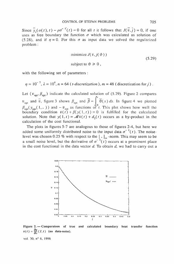
Let v >fi ) iridicate the calculated solution of (5.29). Figure 2 compares
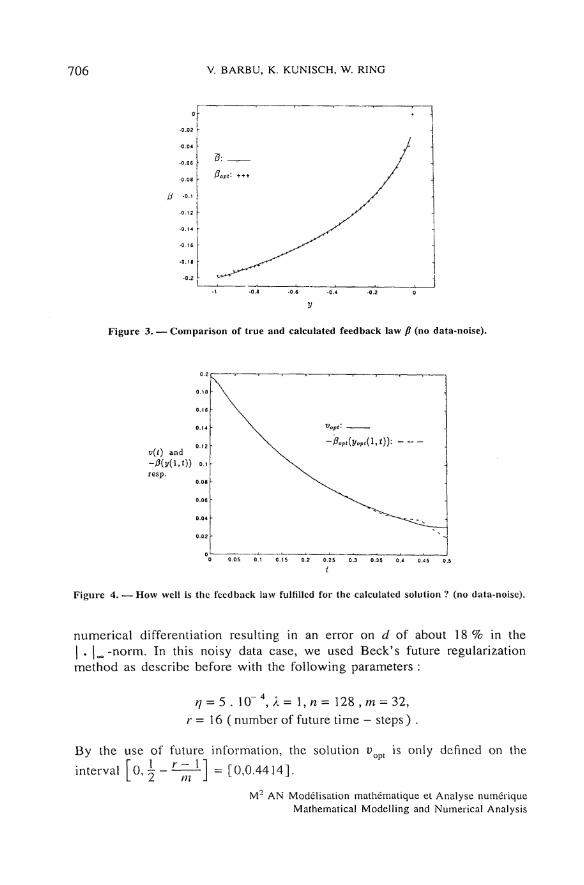
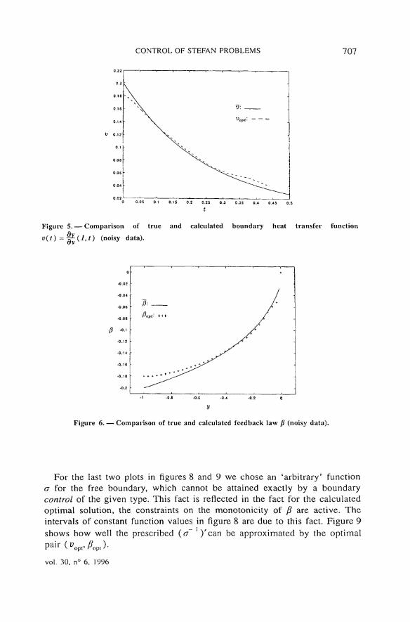
i; and t>, figure 3 shows /?opL and fi = I -Q{s)ds. In figure 4 we plottedv 0
Po [(-VopL 1» • ) ) anc* " yopi a s Onctions of t. This plot shows how well theboundary condition v(t) + fi(y( 1, r) ) = 0 is fulfilled for the calculatedsolution. Note that y( 1, t) = d$v(t) + d2(t) occurs as a by-product in thecalculation of the cost functional.
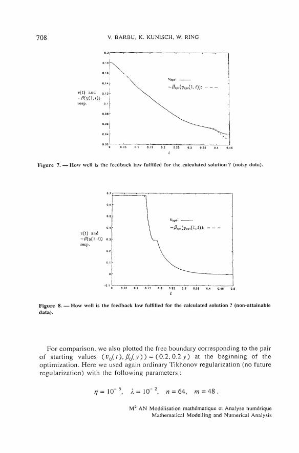
The plots in figures 5-7 are analogous to those of figures 2-4, but hère weadded some uniformly distributed noise to the input data a~ \t). The noise-level was chosen 0.25 % with respect to the | . 1 -norm. This may seem to bea small noise level, but the derivative of a~ l(t) occurs at a prominent placein the cost functional in the data vector d. To obtain d, we had to carry out a
0.22 f
Figure 2. — Comparaison of true and calculated boundary heat transfer function
u(O = ! * ( 7 , O (no data-noise).
vol. 30, n° 6, 1996
706 V. BARBU, K. KUNISCH, W. RING
0
-0.02
-0.04
-0.06
-o.os
0 -o.i
-0.12
-0.14
-0.16
0: fPept'- + + + y
y
•0.8 -0.6 -0.4 .0.2
y
Figure 3. — Comparison of true and calculated feedback law fi (no data-noise).
Figure 4. •— How well is the feedback law fulfilled for the calculated solution ? (no data-noise).
numerical differentiation resulting in an error on d of about 1 8 % in the| . l^-norm. In this noisy data case, we used Beck's future regularizationmethod as describe before with the following parameters :
rj = 5 . 1(T4, Â= l , n = 128, m = 32,r — 16 ( number of future time — steps ) .
By the use of future information, the solution vopt is only defined on the
interval [ o ^ - ^ 1 ^ 1 ] = [0,0.4414].
M2 AN Modélisation mathématique et Analyse numériqueMathematical Modelling and Numerica! Analysis
CONTROL OF STEFAN PROBLEMS 707
Figure 5. — Comparison of true and calculated boundary heat transfer function
i>(O = § * ( ' . ' ) (noisy data).
Figure 6. — Comparison of true and calculated feedback law /? (noisy data).
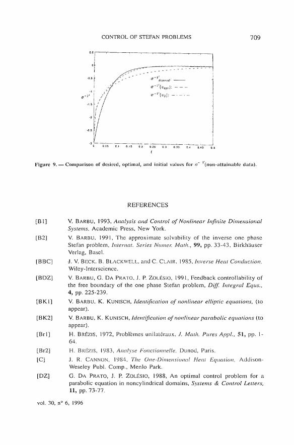
For the last two plots in figures 8 and 9 we chose an 'arbitrary' functiona for the free boundary, which cannot be attained exactly by a boundarycontroï of the given type. This fact is reflected in the fact for the calculatedoptimal solution, the constraints on the monotonicity of ƒ? are active. Theintervals of constant function values in figure 8 are due to this fact. Figure 9shows how well the prescribed (rr~ )'can be approximated by the optimal
vol. 30, n° 6, 1996
708 V. BARBU, K. KUNISCH, W. RING
O 0.0 5 0.1 0.15 0.2 0.25 0.3 0.35 0.4 0.45
Figure 7. — How wcll is the feedback law fulfilled for the calculatcd solution ? (noisy data).
v(t) and- /resp.
' • ' [4
0 0.05 0.1 0.15 0.2 0.25 0.3 0.35 0.4 0.4 5 0.5
t
Figure 8. — How well is the feedback law fulfilled for the calculated solution ? (non-attainabledata).
For comparison, we also plotted the free boundary eorresponding to the pairof starting values ( vo(t), fJQ( y) ) = (0.2, 0.2 y) at the beginning of theoptimization. Here we used again ordinary Tikhonov regularization (no futureregularization) with the following parameters :
0" 5= 10" 5, A = 10" 2, n = 64, m = 48 .
M2 AN Modélisation mathématique et Analyse numériqueMathematica! Modelling and Numerical Analysis
CONTROL OF STEFAN PROBLEMS 709
0 ° 0 5 o t 0.15 0.2 0.25 0.3 0.35 0.4 0.45 '" 0.5
t
Figure 9. — Comparison of dcsircd, optimal, and initial values for a ' (non-uttainablc data).
REFERENCES
[BI] V. BARBU, 1993, Analysis and Control of Nonlinear Infinité Diniensionai
Systems, Academie Press, New York.
[B2] V. BARBU, 1991, The approximate solvabihty of the inverse one phaseStefan problem, Internat. Series Numer. Math., 99, pp. 33-43, BirkhauserVerlag, Bascl.
[BBC] J. V. BECK, B. BLACKWELL, and C. CLAIR, 1985, Inverse Heat Conduction,Wiley-Interscience.
[BDZ] V. BARBU, G. DA PRATO, J. P. ZOLÊSIO, 1991, Feedback controllability of
the free boundary of the one phase Stefan problem, Diff. Intégral Eqiis.,4, pp. 225-239.
[BK1] V. BARBU, K. KUNISCH, Identification of nonlinear elliptic équations, (toappear).
[BK2] V. BARBU, K. KUNISCH, Identification of nonlinear parabolic équations (toappear).
[BrI] H. BRÉZIS, 1972, Problèmes unilatéraux, J. Math. Pures AppL, 51, pp. 1-
64.
[Br2] H. BRÉZIS, 1983, Analyse Fonctionnelle, Dunod, Paris.
[C] J. R. CANNON, 1984, The One-Dimensional Heat Equation, Addison-Weseley Publ. Comp., Menlo Park.
[DZ] G. DA PRATO, J. P. ZOLÉSIO, 1988, An optimal control problem for aparabolic équation in noncylindrical domains, Systems & Control Letters,11, pp. 73-77.
vol. 30, n° 6, 1996
710 V. BARBU, K. KUNISCH, W. RING
[GLS] G RI PEN BERG, S. LONDEN, and STAFFANS, 1990, Volterra intégrai and Fitnc-tional Equations, Cambridge University Press.
[HN] K. H. HOFFMANN, M. NiEZGODKA, 1990, Control of evolutionary f re e boiin-dary problems, in F ree Boundary Probtems : Theory and Applications,pp. 439-450, K. H. Hoffmann and J. Sprckels, eds., Pitman Research Notes inMathematics 186, Longman, London.
[HS] K. H. HOFFMANN, J. SPREKELS, 1982, Real time control of the free boundaryin a two phase Stefan problem, Numerical Functional Anal. Optimiz, 5,pp. 47-76.
[KMP] K. KUNISCH, K. MURPHY, and G. PE1CHL, Estimation of the conductivity in theone-phase Stefan problem : Basic results, to appear in Bolletino Unione Mat.Italiana.
[La] P. K. LAMM, Future-sequential regularization methods for ill-posed Volterra
équations, to appear in J. Math. Anal, and Appl.
[Li] J. L. LIONS, 1969, Quelques Methodes de Résolutions de Problèmes aux
Limites Nonlinéaires, Dunod, Paris.
[PW] H. PROTER, H. WEINBERGER, 1983, The Maximum Principle, Springer-Verlag,Berlin.
M2 AN Modélisation mathématique et Analyse numériqueMathematical Modelling and Numerical Analysis


![IJMPERD - Comparative Study by Numerical Investigation of ......0.25 MWCNTs-0.035 GNPs/water hybrid nanofluids. Kaska et al. [12] enhanced the heat transfer of water by using alumina](https://img.pdfslide.fr/doc/110x75/60b9c51307e90c51185cd97d/ijmperd-comparative-study-by-numerical-investigation-of-025-mwcnts-0035.jpg)