DYNAMIC ANALYSIS OF ISOTROPIC AND … ANALYSIS OF ISOTROPIC AND LAMINATED REINFORCED COMPOSITE PLATES ... 5.2 Modal analysis of plate totally ... Laminated plate simply supported …

UNIVERSITÉ DE MONTRÉAL

DYNAMIC ANALYSIS OF ISOTROPIC AND LAMINATED REINFORCED

COMPOSITE PLATES SUBJECTED TO FLOWING FLUID

ALIREZA JALALI

DÉPARTEMENT DE GÉNIE MÉCANIQUE

ÉCOLE POLYTECHNIQUE DE MONTRÉAL

MÉMOIRE PRÉSENTÉ EN VUE DE L’OBTENTION

DU DIPLÔME DE MAÎTRISE ÈS SCIENCES APPLIQUÉES

(GÉNIE MÉCANIQUE)

Avril 2012

© Alireza Jalali, 2012

UNIVERSITÉ DE MONTRÉAL

ÉCOLE POLYTECHNIQUE DE MONTRÉAL

Ce mémoire intitulé:

DYNAMIC ANALYSIS OF ISOTROPIC AND LAMINATED REINFORCED

COMPOSITE PLATES SUBJECTED TO FLOWING FLUID

Présenté par : JALALI Alireza

en vue de l’obtention du diplôme de : Maîtrise ès Sciences Appliquées

a été dûment accepté par le jury d’examen constitué de :

M. BALAZINSKI, Marek, Ph.D., président

M. LAKIS, Aouni A, Ph.D., membre et directeur de recherche

M. HOJJATI, Mehdi, Ph.D., membre

iii

DEDICATION

I lovingly dedicate this thesis to my wife and my parents, who supported me each step of the

way.

iv

ACKNOWLEDGEMENT

I would like to show my gratitude to my supervisor, Aouni. A. Lakis, to support me in this

way. I would also like to thank my uncle, Shahriar, and his family for their support. Also I am

heartily thankful to my friend, Dr. M. H. Toorani, whose encouragement, guidance and

support from the initial to the final level enabled me to develop an understanding of the

subject.

My very special thanks to the two guys whom I owe everything I am today, my parents. Their

unwavering faith and confidence in my abilities and in me is what has shaped me to be the

person I am today. Thank you for everything.

v

RÉSUMÉ

Dans ce travail nous examinons le comportement dynamique d’une structure en composite,

symétriquement élastique, et d’une plaque anisotrope soumise à un flux de fluide non-

visqueux et incompressible. Pour une modélisation mathématique, une combinaison entre la

méthode des éléments finis ainsi que la théorie des plaques minces a été utilisée. Pour définir

la propriété des composites, un élément rectangulaire anisotrope a été utilisé. La plaque est

composée de N couches qui peuvent être fabriquées de fibres unidirectionnelles avec

différentes matrices. Ces fibres pourraient être continues, discontinues ou dans un mode

aléatoire. L’inertie, la force de Coriolis et la force centrifugeuse du fluide introduisent une

pression dynamique qui est modélisée en utilisant la fonction du potentiel de Bernoulli. La

condition d’imperméabilité entre la plaque et le fluide est aussi prise en compte. Les matrices

de masse et de rigidité pour chaque élément de la plaque ont été calculées par une intégration

analytique exacte. Une corrélation assez proche entre la théorie présentée avec les approches

expérimentales et Ansys (logiciel d’éléments finis) a été démontrée.

vi

ABSTRACT

In situations of fluid and structure, the dynamic behavior of the structure may vary. Structures

can lose their stability due to fluid/solid interaction.

Modal analysis and the dynamic behavior of elastically symmetrical laminated composites as

well as isotropic plates subjected to an incompressible, inviscid flowing fluid are studied in

this work using shell and thin plate theories. The effect of stacking sequence and boundary

conditions on the natural frequency and static instability of the model are studied. Shear

deformation effect is not taken into account. For mathematical modeling, a combination of a

hybrid finite element method and classic laminate thin plate theory are used. The finite

element is defined as a rectangular thin laminated composite plate with four nodes. Each node

has six degrees of freedom to cover all possible movements. The plate consists of N layers

that could be made of unidirectional fibers in different matrices and these fibers could be

continuous, discontinuous or random modes but in this study in all the examples, models

consist of continuous fibers. Inertia, Coriolis and centrifugal fluid forces introduce a dynamic

pressure field which is modeled using a velocity potential function and Bernoulli’s equation.

This pressure field is a function of the nodal displacement. The impermeability condition

between the plate and the fluid is also taken into account. Mass and stiffness matrices for each

element of the plate are calculated by exact analytical integration using MATLAB

programming software. Close agreement between the presented theory and other sources such

as commercial finite element software (ANSYS) and experimental approaches is

demonstrated.

vii

TABLE OF CONTENTS

DEDICATION ........................................................................................................................... iii

ACKNOWLEDGEMENT ......................................................................................................... iv

RÉSUMÉ .................................................................................................................................... v

ABSTRACT ............................................................................................................................... vi

TABLE OF CONTENTS .......................................................................................................... vii

LIST OF TABLES ...................................................................................................................... x

LIST OF FIGURES ................................................................................................................... xi

LIST OF ACRONYMS AND ABREVIATIONS ................................................................... xiii

INTRODUCTION ...................................................................................................................... 1

CHAPTER 1 LAMINATED COMPOSITE MATERIAL .............................................. 5

1.1 Introduction ..................................................................................................................... 5

1.2 Definitions....................................................................................................................... 5

CHAPTER 2 STRAIN-DISPLACEMENT AND STRESS-STRAIN RELATIONS ..... 10

2.1 General strain-displacement relations ................................................................................. 10

2.2 Strain-displacement relations for laminated composite rectangular plates ......................... 13

2.3 Introducing local and global coordinate system for finite element at Kth lamina ............... 14

2.4 Stress-strain relations of the Kth lamina in local coordinate system (α, β and γ or 1, 2,3) . 15

2.5 Stress-strain relations of the Kth lamina in global coordinate system (x,y and z) ............... 16

CHAPTER 3 SOLID FINITE ELEMENT MODEL ....................................................... 20

3.1 Structure modeling .............................................................................................................. 20

3.2 Equilibrium equations in term of displacement .................................................................. 20

3.3 Displacement functions ...................................................................................................... 21

viii

3.4 Linear Strain-displacement relations .................................................................................. 24

3.5 Constitutive equations ......................................................................................................... 24

CHAPITRE 4 DYNAMIC FLUID-STRUCTURE INTERACTIONS .......................... 26

4.1 Assumption ......................................................................................................................... 26

4.2 Equation of motion ............................................................................................................. 26

4.3 Development of fluid matrices............................................................................................ 27

4.3.1 Solid-fluid model with infinite fluid level .............................................................. 30

4.3.2 Solid-fluid model with finite fluid level ................................................................. 31

4.3.3 Solid-fluid model surrounded by parallel rigid wall ............................................... 32

4.3.4 Determination of force induced by fluid dynamic pressure .................................... 34

4.4 Global matrices and Eigenvalue solution ........................................................................... 37

CHAPTER 5 RESULTS AND DISCUSSIONS.............................................................. 39

5.1 Modal analysis of laminated plate ...................................................................................... 39

5.1.1 Essential number of elements for an accurate results ............................................... 39

5.1.2 Compare present method with other investigations and commercial software ........41

5.1.3 Effect of boundary condition on natural frequency of orthotropic plate .................. 43

5.1.4 Effect of different stacking sequence of laminas on natural frequency of orthotropic

plates ......................................................................................................................... 45

5.2 Modal analysis of plate totally submerged in fluid ............................................................. 47

5.2.1 Example 1: Natural frequency of submerged isotropic plate.................................... 47

5.2.2 Example 2: Natural frequency of laminated plate in air (vacuo) .............................. 48

5.2.3 Example 3: Natural frequency of laminated plate on free fluid surface and totally

submerged situations ................................................................................................ 50

5.2.4 Example 4: Comparison between the effect of fluid on natural frequency of

isotropic plate and laminated plate ........................................................................... 52

ix

5.3 Stability analysis of plate subjected to the flowing fluid .................................................... 53

1.1 Example 1:Laminated plate clamped on two opposite edges coupled to flowing fluid 53

1.2 Example 2: Laminated plate with different stacking sequences, clamped on two

opposite edgescoupled to flowing fluid ........................................................................ 54

5.4 Effect of boundary condition on critical fluid velocity ....................................................... 57

5.4.1 Example 1: Laminated plate simply supported on two opposite edges coupled to

flowing fluid ............................................................................................................. 57

5.4.2 Example 2: Cantilever laminated plate coupled to flowing fluid ........................... 58

CHAPITRE 6 CONCLUSION AND FUTURE WORK ............................................... 60

REFERENCES ......................................................................................................................... 62

APPENDIX A ........................................................................................................................... 65

APPENDIX B ........................................................................................................................... 68

x

LIST OF TABLES

Table 5.1: Natural frequency (Hz) of totally clamped laminated plate which discretized to

different number of finite elements. ........................................................................ 40

Table 5.2: Natural frequency (Hz) for graphite/epoxy1 totally clamped at its four edges. .... 41

Table 5.3: Natural frequency (Hz) for steel plate simply supported at its four edges ............ 42

Table 5.4: Natural frequency (Hz) for graphite/epoxy1 in different boundary conditions ..... 44

Table 5.5: Natural frequency (Hz) for graphite/epoxy with five different stacking sequences45

Table 5.6: Frequencies (Hz) for Isotropic cantilever plate totally submerged in water. ........ 48

Table 5.7: Natural frequency (Hz) for case 1, square (0.076m 0.076m) cantilever 8-ply

graphite/epoxy [45/-45/-45/45] sym in air (vacuo) ................................................. 49

Table 5.8: Natural frequency (Hz) for case 2, Rectangular (0.152m 0.076m) cantilever 8-ply

graphite/epoxy [45/-45/-45/45]sym in air (vacuo) .................................................. 49

Table 5.9: First natural frequency (Hz) for Rectangular (0.152m 0.076m) cantilever 8-ply

graphite/epoxy [45/-45/-45/45]sym on fluid free surface and totally submerged in

fluid. ...................................................................................................................... 51

Table 5.10: First three natural frequencies (Hz) of isotropic and laminated cantilever plate in

air and water. ........................................................................................................ 52

Table 5.11: Critical fluid velocity (m/s) for first three modes of plates clamped on two

opposite edges subjected to flowing fluid ............................................................ 55

Table 5.12: Critical fluid velocity (m/s) for first three modes of Graphite/epoxy1 for different

boundary conditions ............................................................................................. 59

xi

LIST OF FIGURES

Figure 1.1: Composite plate with different layers and different thicknesses ............................. 6

Figure 1.2: Unidirectional oriented fiber composite .................................................................. 7

Figure 1.3: Typologies of fiber-reinforced composite materials ............................................... 8

Figure 2.1: a) shell element, b) shell coordinate system .......................................................... 11

Figure 2.2: Rectangular laminated composite plate ................................................................. 13

Figure 2.3: Global and local coordinate systems for laminated composite plates ................... 14

Figure 3.1: Plate geometry, coordinate systems and finite element discretization .................. 20

Figure 4.1: Solid-fluid model with infinite level of fluid ........................................................ 30

Figure 4.2: Solid-fluid model with finite level of fluid ........................................................... 31

Figure 4.3: Laminated composite plate subjected to following fluid and surrounded by rigid

wall ........................................................................................................................ 32

Figure 4.4: The plate totally submerged in flowing fluid ........................................................ 33

Figure 5.1: The five first natural frequencies of the totally clamped laminated plate as a

function of number of elements. .......................................................................... 40

Figure 5.2: First five mode shapes of graphite/epoxy1 totally clamped at its four edges. a)

First mode. b) Second mode. c) Third mode. d) Fourth mode. e) Fifth mode. ..... 42

Figure 5.3: First five natural frequencies (Hz) for graphite/epoxy1 under different boundary

conditions .............................................................................................................. 44

Figure 5.4: First two natural frequencies (Hz) for graphite/epoxy with different stacking

sequences ............................................................................................................. 46

Figure 5.5: Cantilever square isotropic plate totally submerged in fluid. ................................ 47

Figure 5.6: Cantilever rectangular laminated plate in air (vacuo) ........................................... 49

xii

Figure 5.7: a) Cantilever laminated plate on the free surface of fluid. b) Cantilever laminated

plate totally submerged in fluid. ............................................................................ 50

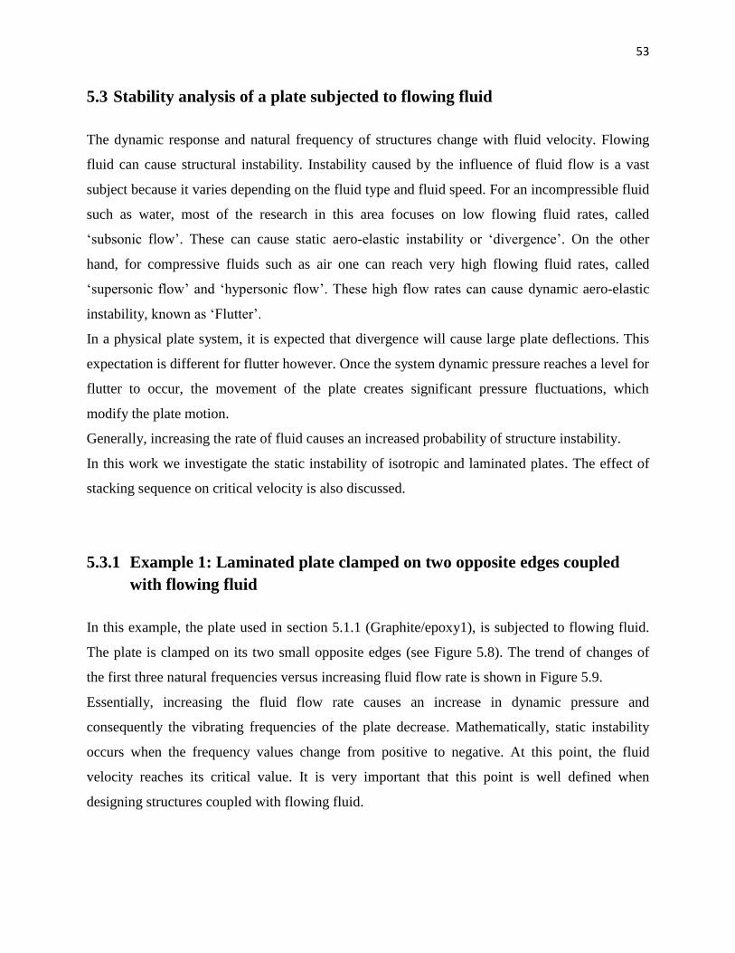
Figure 5.8: Graphite/epoxy1 clamped on two opposite edges faced to flowing fluid ............. 54

Figure 5.9: Changes of frequency (Hz) versus fluid velocity (Ux (m/s)) for a Graphite/epoxy1

clamped on two opposite edges faced to flowing fluid ......................................... 54






simply supported on two opposite edges faced to flowing fluid ......................... 57


cantilever on small edge faced to flowing fluid ................................................... 58

xiii

LIST OF ACRONYMS AND ABREVIATIONS

CLPT Classical laminate thin plate theory

HFEM Hybrid finite element method

FEM Finite element method

FEA Finite element analysis

HFEM Hierarchical Finite Element Method

SS Simply Supported

C Clamped

F Free

Sym Symmetry

Cr Critical

FSDT First-order shear deformation theory

HSDT Higher-order shear deformation theory

FSI Fluid-structure-interaction

RBF Radial basis function

1

INTRODUCTION

Systems of shells and plates subjected to flowing fluid are used extensively in modern

engineering designs in a variety of industries. Some examples are; ship building, nuclear,

aerospace and aeronautical industries, pipe line systems in petroleum and petrochemical

industries and car manufacturing.

Many investigations have been undertaken to study the dynamic response of structures subjected

to fluid. Some approximate methods such as the beam function, Galerkin‘s Method, Rayleigh-

Ritz Method, etc were proposed to determine the change of natural frequencies during fluid-solid

interaction problems. Although these approximate methods remain useful, recent improvements

in technology can now be applied to provide exact solutions of the dynamic behavior of fluid-

structure systems. These methods deepen our understanding of the fluid-structure interaction

(FSI) problem.

In most fluid-structure-interaction models, a condition exists involving a high rate of fluid flow

versus low plate thickness. Under these conditions, if the thickness is much less than the length

of the plates or shells, the structure becomes very susceptible to collapse. From this point of

view, controlling and decreasing the dynamic stress and /or vibration amplitudes are the final

goals. Since these are related to the dynamic response of the system, some of the most important

factors that should be studied are the modal analysis and dynamic behavior of these systems.

In general, fluid interaction decreases the natural vibration frequencies of the structure. There

are many publications that describe how this phenomenon can occur for different material types,

geometries and various situations.

In recent years, application of composite materials has increased due to the opportunity to

develop structures with high strength-to-weight and stiffness-to-weight ratios. Plates of

composite materials are also characterized by anisotropy and out-of-plane shear rigidity. This

combination of characteristics of composite materials has led to the initiation of significant

investigation work in the aircraft and aerospace industries.

A large number of studies have been published involving natural frequency and modal analysis

of systems of shells and plates. In particular, there are many investigations for isotropic plates.

For example Leissa [1] conducted an extensive study on the vibration of plates with various

geometries fabricated from isotropic and anisotropic materials. Also in an anisotropy context,

2

Reddy [2] uses the finite element method and the first shear deformation theory to present a

clear, detailed analysis of free vibration of simply-supported antisymmetric and angle-ply

laminated plates. Han [3] extended the p-version finite element method to evaluate the natural

frequency of symmetrical laminated rectangular plates and Hsu [4] studied the free vibration of

both isotropic and orthotropic rectangular plates with different boundary conditions. He used the

differential quadrature method in his work. Wanmin Han and M. Petyt [3] used a hierarchical

finite element method to study the vibration characteristics of symmetrically laminated

rectangular plates. Modal analysis of symmetric laminated composite plates is studied by Xiang,

S., Wang, et al [5] using other methods. They used trigonometric shear deformation theory for

laminated beams to drive the differential governing equations of the plate. They also used a

meshless collection method based on the inverse multi-quadric radial basis function (RBF) to

find the natural frequency of structures.

Former works considering the effect of fluid on plate vibration were carried out by Lamb [6]. He

used Rayleigh‘s method to calculate the modes of a circular isotropic plate totally-clamped with

fluid on one side. Fu and Price [7] performed an analytical study of the vibration behavior of

cantilever plates partially or totally immersed in fluid. The effects of free surface, length and

depth of the plate on its dynamic characteristics were explained using a combination of the finite

element method and a singularity distribution panel approach. To study the interaction between

cylindrical thin shells and stationary liquid, Lakis and Paidoussiss [8] developed a new method

incorporating a hybrid finite element. Also, a very complete study of fluid-structure interaction

involving flowing fluid and thin structures was conducted by Paidoussiss [9].

For rectangular plates, Lindholm et al [10] presented valuable experimental data describing the

dynamic behavior of cantilever plates in water and air. Eric Sharbonneau [11] presented a

method for dynamic analysis of thin, elastic, isotropic, rectangular plates in a vacuo or

submerged in a fluid. He also investigated the effect of different boundary conditions and plate

geometry, together with the depth of submergence. His method combined hybrid finite element

theory and classic thin plate theory. He provided the mass and stiffness matrices for the plate

element and introduced a fluid mass matrix describing the interaction of the fluid pressure over

the plate element. The results using this method are in good agreement with those obtained by

others.

3

The equations of motion of anisotropic plates and shells have been studied by Toorani [12]. This

investigation again used the hybrid finite element method developed by Lakis and Paidoussiss

[8]. His bibliography is very inclusive, with more than 150 references. He developed the general

equations of anisotropic plates and shells for various geometries with respect to shear

deformations, rotary inertia and initial curvature effects. Following this, Toorani and Lakis [13]

conducted a dynamic analysis of anisotropic cylindrical shells subjected to internal and/or

external flowing fluid using the hybrid finite element approach. The equations of motion for

cylindrical shells used in their work are based on the previous work done by Toorani [12] and

includes consideration of shear transverse deformations.

To investigate the vibration of rectangular plates, a hybrid method was developed by Kerboua

and Lakis [14]. This method is a combination of the finite element method and Sander‘s shell

theory in which the in-plane and membrane displacement components are taken into account.

A valuable experimental and analytical study was done by Haddara [15] on the dynamic

response of submerged flat plates. He observed the effect of boundary conditions and fluid depth

on the plates. Pal, Sinha and Bhattacharyya [16] conducted a finite element analysis to determine

dynamic characteristics such as the natural frequency, amplitude and period of response of

isotropic and composite plates in a vacuo and submerged in water. They did not take into

account the effect of viscous damping in their work.

Nguen-Fuk-Nin [17] investigated flutter of an orthotropic cantilevered plate with two stiffener

ribs. They used elastic strain energy in the Lagrange equation and studied the influence of

Poisson ratio on the critical flow velocity. Santini [18] performed an analytical approach and a

span-wise finite element solution to describe the dynamic behaviour of a cantilever wing

structure simulated using an anisotropic swept plate. Using numerical examples he showed the

effect of sweep and anisotropicity on the frequencies and modes. He described a trapezoidal

platform wing and used the Hamilton principle to develop the structural equations. For analysis

of the dynamic behavior of the wing (plate), he utilized the dynamic response in harmonic time-

variation.

Some recent investigations have been done by Kerboua and Lakis [19-21] on the dynamic

behavior of a plate submerged in fluid and floating on its free surface. These studies also include

modeling of plates subjected to flowing fluid under various boundary conditions. The critical

fluid velocity is calculated for an isotropic plate under different boundary conditions. Critical

4

velocity is also calculated for a plate bounded with rigid or elastic parallel walls and a plate

submerged in a fluid of infinite dimensions.

In the present work, the characteristics of different types of laminated materials (fibers and

matrices) are explained, and then the general equations of motion for a composite rectangular

plate are presented. Finally, a solid-fluid finite element model is developed to study the dynamic

response of a balanced symmetric laminated [22] rectangular plate subjected to potential flow.

This investigation allows us to obtain low and high frequencies in a fluid-structure situation

using only a few finite elements. This exact solution is obtained at reduced computer time and

cost compared to other conventional methods.

5

CHAPTER 1 LAMINATED COMPOSITE MATERIAL

1.1 Introduction

Recent technological improvements are providing designers with a larger range of materials to

choose from depending on their particular application. In many cases, composite materials are a

preferred choice compared to materials such as steel and aluminum because they can better meet

the needs of these applications.

―Composite materials are those formed by combining two or more materials on a macroscopic

scale such that they have better engineering properties than conventional materials, for example,

metals‘‘ [23].

―Major constituents in composite materials are fiber-reinforced composite materials. Fiber-

reinforced composite materials consist of fibers of high strength and modulus embedded in or

bonded to a matrix with distinct interfaces (boundaries) between them. In this form, both fibers

and matrix retain their physical and chemical identities, yet they produce a combination of

properties that cannot be achieved with either of the constituents acting alone‘‘[22].

Among the various different composite materials available today, laminated layer materials are

the most frequently applied in industry.

1.2 Definition

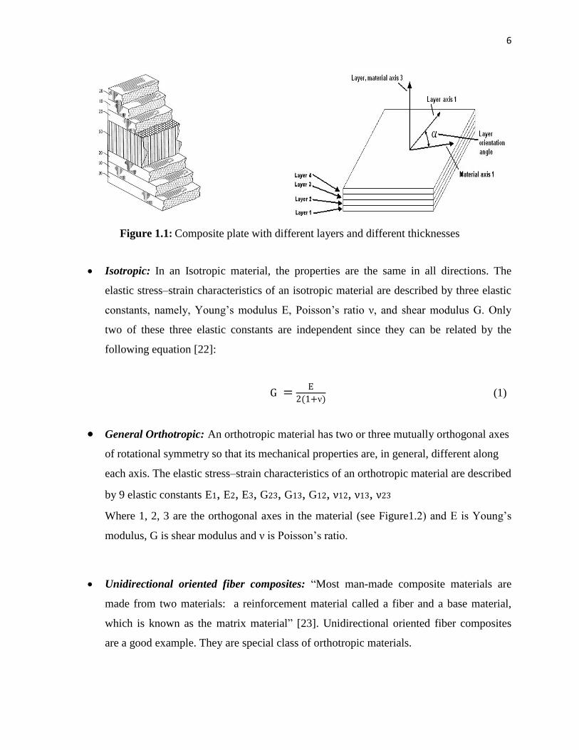
Laminated plates are made of N different layers of various thicknesses (see Figure1.1). Each

layer is called a lamina. Laminas can be classified in three different categories: Isotropic,

Unidirectional oriented fiber composites and General Orthotropic

6

Figure 1.1: Composite plate with different layers and different thicknesses

Isotropic: In an Isotropic material, the properties are the same in all directions. The

elastic stress–strain characteristics of an isotropic material are described by three elastic

constants, namely, Young‘s modulus E, Poisson‘s ratio ν, and shear modulus G. Only

two of these three elastic constants are independent since they can be related by the

following equation [22]:

ν (1)

General Orthotropic: An orthotropic material has two or three mutually orthogonal axes

of rotational symmetry so that its mechanical properties are, in general, different along

each axis. The elastic stress–strain characteristics of an orthotropic material are described

by 9 elastic constants E1, E2, E3, G23, G13, G12, 12, 13, 23

Where 1, 2, 3 are the orthogonal axes in the material (see Figure1.2) and E is Young‘s

modulus, G is shear modulus and ν is Poisson‘s ratio.

Unidirectional oriented fiber composites: ―Most man-made composite materials are

made from two materials: a reinforcement material called a fiber and a base material,

which is known as the matrix material‖ [23]. Unidirectional oriented fiber composites

are a good example. They are special class of orthotropic materials.

7

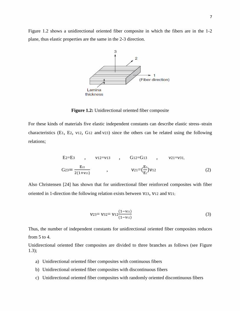
Figure 1.2 shows a unidirectional oriented fiber composite in which the fibers are in the 1-2

plane, thus elastic properties are the same in the 2-3 direction.

Figure 1.2: Unidirectional oriented fiber composite

For these kinds of materials five elastic independent constants can describe elastic stress–strain

characteristics (E1, E2, 12, G12 and 23) since the others can be related using the following

relations;

E2=E3 , 12= 13 , G12=G13 , 21= 31,

G23

, 21=

12 (2)

Also Christensen [24] has shown that for unidirectional fiber reinforced composites with fiber

oriented in 1-direction the following relation exists between 23, 12 and 21;

23= 32= 12

(3)

Thus, the number of independent constants for unidirectional oriented fiber composites reduces

from 5 to 4.

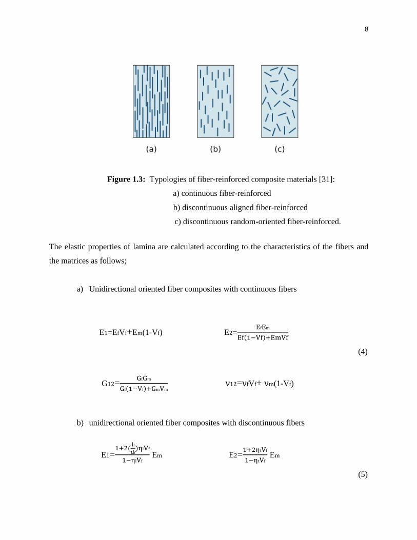
Unidirectional oriented fiber composites are divided to three branches as follows (see Figure

1.3);

a) Unidirectional oriented fiber composites with continuous fibers

b) Unidirectional oriented fiber composites with discontinuous fibers

c) Unidirectional oriented fiber composites with randomly oriented discontinuous fibers

8

Figure 1.3: Typologies of fiber-reinforced composite materials [31]:

a) continuous fiber-reinforced

b) discontinuous aligned fiber-reinforced

c) discontinuous random-oriented fiber-reinforced.

The elastic properties of lamina are calculated according to the characteristics of the fibers and

the matrices as follows;

a) Unidirectional oriented fiber composites with continuous fibers

E1=EfVf+Em(1-Vf) E2=

(4)

G12=

12= fVf+ m(1-Vf)

b) unidirectional oriented fiber composites with discontinuous fibers

E1=

Em E2=

Em

(5)

http://en.wikipedia.org/wiki/File:Fiber-reinforced_composites_tipology.svg

9

G12=

Gm 12= fVf + mVm

c) Unidirectional oriented fiber composites with randomly oriented discontinuous

fibers

Erandom=

random=

(6)

Grandom=

where E1, E2 used in (c), are the same as in (b)

= (

⁄ )

(

⁄ ) ( ⁄ )

= (

⁄ )

(

⁄ ) =

(

⁄ )

(

⁄ ) (7)

= longitudinal modulus for a fiber. = matrix volume fraction.

= longitudinal modulus for a matrix. = length of fiber

= fiber volume fraction = fiber diameter

= fiber shear modulus matrix shear modulus

fiber matrix

10

CHAPTER 2 STRAIN-DISPLACEMENT AND STRESS-STRAIN

RELATIONS

2.1 General strain-displacement relations

For general shell element as shown in Figure 2.1, The normal and shear strains can be related to

the displacement vector component as [25];

.

√ /

∑

√

(8)

√ 0

.

√ /

.

√ /1

where , and are the curvilinear coordinates of the surface, the components of the

displacement vector and geometrical scale factor quantities. They are defined for thin plate and

shell applications as follows:

(9)

(

)

(

)

where and are the curvature radius and the Lame‘s parameters. U, V and W are the

displacement vectors and are the thickness coordinates.

The displacement components are presented by following equations;

11

(10)

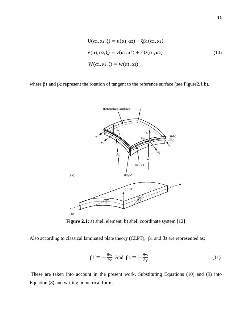
where and represent the rotation of tangent to the reference surface (see Figure2.1 b).

Figure 2.1: a) shell element, b) shell coordinate system [12]

Also according to classical laminated plate theory (CLPT), and are represented as;

And

(11)

These are taken into account in the present work. Substituting Equations (10) and (9) into

Equation (8) and writing in metrical form;

12

(

) 0 0 0 0 0

0

(

) 0 0 0 0 τ1

(

)

(

) 0 0 + 𝜉 τ2 (12)

0 0 0

(

) 0 0

0 0 0 0 0

(

)

where;

(

)

(

)

;

(

)

(

)

(

)

(

)

;

(

)

(

)

(

)

(

) ;

(

)

(

) (12.a)

(

)

(

) ;

(

)

(

)

(

)

;

(

)

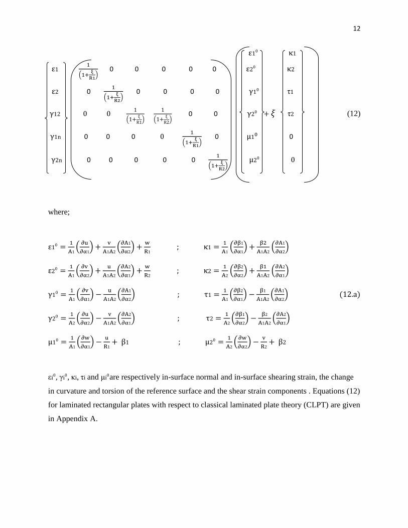
, , τ and are respectively in-surface normal and in-surface shearing strain, the change

in curvature and torsion of the reference surface and the shear strain components . Equations (12)

for laminated rectangular plates with respect to classical laminated plate theory (CLPT) are given

in Appendix A.

13

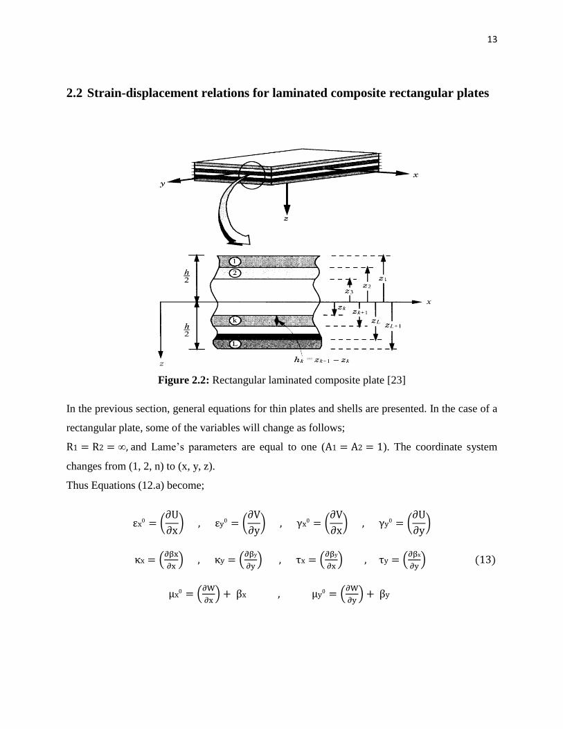
2.2 Strain-displacement relations for laminated composite rectangular plates

Figure 2.2: Rectangular laminated composite plate [23]

In the previous section, general equations for thin plates and shells are presented. In the case of a

rectangular plate, some of the variables will change as follows;

and Lame‘s parameters are equal to one ( ). The coordinate system

changes from (1, 2, n) to (x, y, z).

Thus Equations (12.a) become;

(

) (

) (

) (

)

(

) (

) (

) (

) (13)

(

) , (

)

14

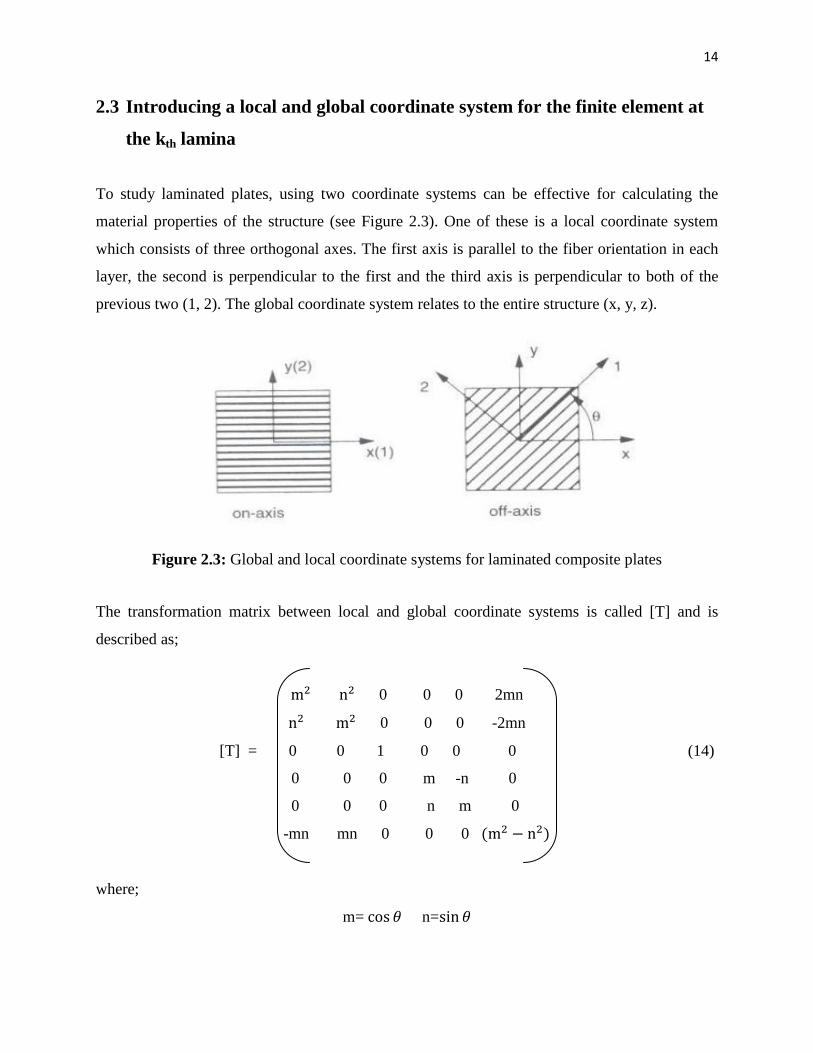
2.3 Introducing a local and global coordinate system for the finite element at

the kth lamina

To study laminated plates, using two coordinate systems can be effective for calculating the

material properties of the structure (see Figure 2.3). One of these is a local coordinate system

which consists of three orthogonal axes. The first axis is parallel to the fiber orientation in each

layer, the second is perpendicular to the first and the third axis is perpendicular to both of the

previous two (1, 2). The global coordinate system relates to the entire structure (x, y, z).

Figure 2.3: Global and local coordinate systems for laminated composite plates

The transformation matrix between local and global coordinate systems is called [T] and is

described as;

0 0 0 2mn

0 0 0 -2mn

[T] = 0 0 1 0 0 0 (14)

0 0 0 m -n 0

0 0 0 n m 0

-mn mn 0 0 0

where;

m= n=

15

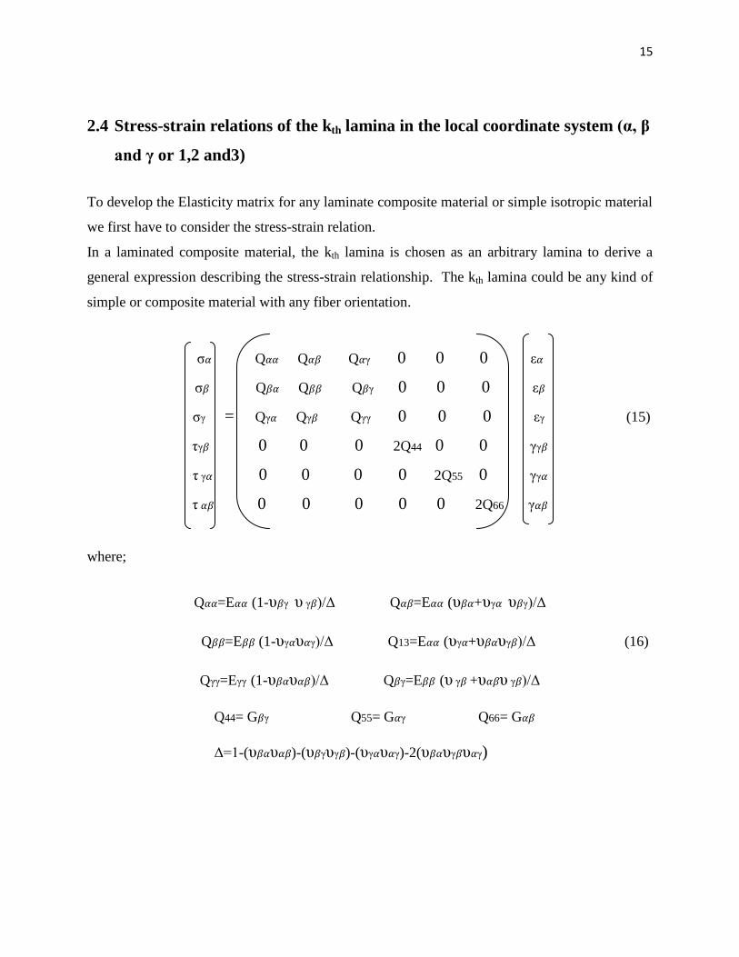
2.4 Stress-strain relations of the kth lamina in the local coordinate system (α, β

and γ or 1,2 and3)

To develop the Elasticity matrix for any laminate composite material or simple isotropic material

we first have to consider the stress-strain relation.

In a laminated composite material, the kth lamina is chosen as an arbitrary lamina to derive a

general expression describing the stress-strain relationship. The kth lamina could be any kind of

simple or composite material with any fiber orientation.

σ𝛼 Q𝛼𝛼 Q𝛼𝛽 Q𝛼 0 0 0 𝛼

σ𝛽 Q𝛽𝛼 Q𝛽𝛽 Q𝛽 0 0 0 𝛽

σ = Q 𝛼 Q 𝛽 Q 0 0 0 (15)

τ 𝛽 0 0 0 2Q44 0 0 𝛽

τ 𝛼 0 0 0 0 2Q55 0 𝛼

τ 𝛼𝛽 0 0 0 0 0 2Q66 𝛼𝛽

where;

Q𝛼𝛼=E𝛼𝛼 (1-υ𝛽 υ 𝛽)/Δ Q𝛼𝛽=E𝛼𝛼 (υ𝛽𝛼+υ 𝛼 υ𝛽 )/Δ

Q𝛽𝛽=E𝛽𝛽 (1-υ 𝛼υ𝛼 )/Δ Q13=E𝛼𝛼 (υ 𝛼+υ𝛽𝛼υ 𝛽)/Δ (16)

Q =E (1-υ𝛽𝛼υ𝛼𝛽)/Δ Q𝛽 =E𝛽𝛽 (υ 𝛽 +υ𝛼𝛽υ 𝛽)/Δ

Q44= G𝛽 Q55= G𝛼 Q66= G𝛼𝛽

Δ=1-(υ𝛽𝛼υ𝛼𝛽)-(υ𝛽 υ 𝛽)-(υ 𝛼υ𝛼 )-2(υ𝛽𝛼υ 𝛽υ𝛼 )

16

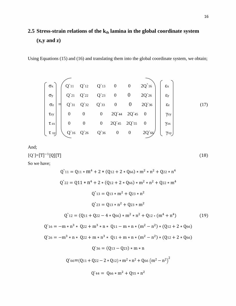
2.5 Stress-strain relations of the kth lamina in the global coordinate system

(x,y and z)

Using Equations (15) and (16) and translating them into the global coordinate system, we obtain;

σx Q`11 Q`12 Q`13 0 0 2Q`16 x

σy Q`21 Q`22 Q`23 0 0 2Q`26 y

σz = Q`31 Q`32 Q`33 0 0 2Q`36 z (17)

τzy 0 0 0 2Q`44 2Q`45 0 zy

τ zx 0 0 0 2Q`45 2Q`55 0 zx

τ xy Q`16 Q`26 Q`36 0 0 2Q`66 xy

And;

[Q`]=[ ] [ ][ ] (18)

So we have;

(19)

=( ) ( )

17

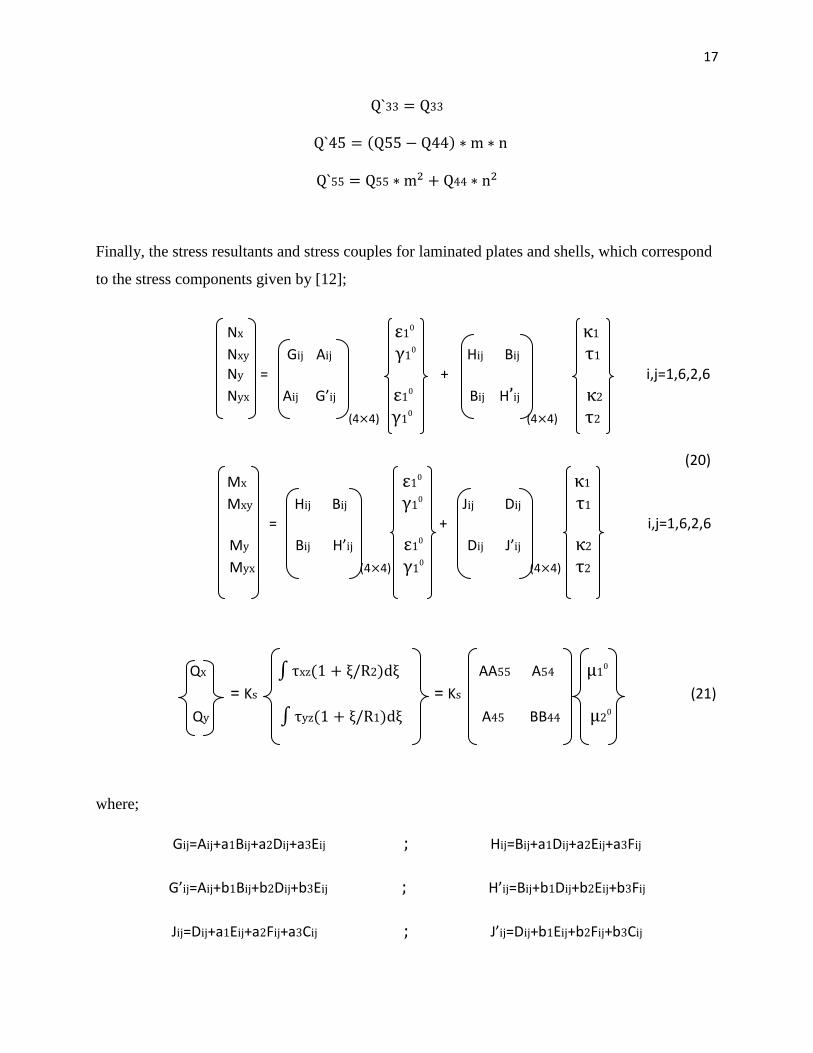
Finally, the stress resultants and stress couples for laminated plates and shells, which correspond

to the stress components given by [12];

Nx

1 Nxy Gij Aij

Hij Bij 1 Ny = + i,j=1,6,2,6 Nyx Aij G’ij

Bij H’ij 2 (4 4)

(4 4) 2

(20) Mx

1 Mxy Hij Bij

Jij Dij 1 = + i,j=1,6,2,6 My Bij H’ij

Dij J’ij 2 Myx (4 4)

(4 4) 2

Qx ∫ AA55 A54

= Ks = Ks (21) Qy ∫ A45 BB44

where;

Gij=Aij+a1Bij+a2Dij+a3Eij ; Hij=Bij+a1Dij+a2Eij+a3Fij

G’ij=Aij+b1Bij+b2Dij+b3Eij ; H’ij=Bij+b1Dij+b2Eij+b3Fij

Jij=Dij+a1Eij+a2Fij+a3Cij ; J’ij=Dij+b1Eij+b2Fij+b3Cij

18

a1=

; b1=

(22)

a2=

; b2=

a3=

; b3=

Aij=∑

; Eij=

∑

Bij=

∑

; Fij=

∑

Dij=

∑

; Cij=

∑

i,j = 1,2,6

AA55=A55+a1B55+a2D55+a3E55 ; BB44= A44+b1B44+b2D44+b3E44

A𝛼𝛽=∑

; B𝛼𝛽=

∑

D𝛼𝛽=

∑

; E𝛼𝛽=

∑

α= 4,5

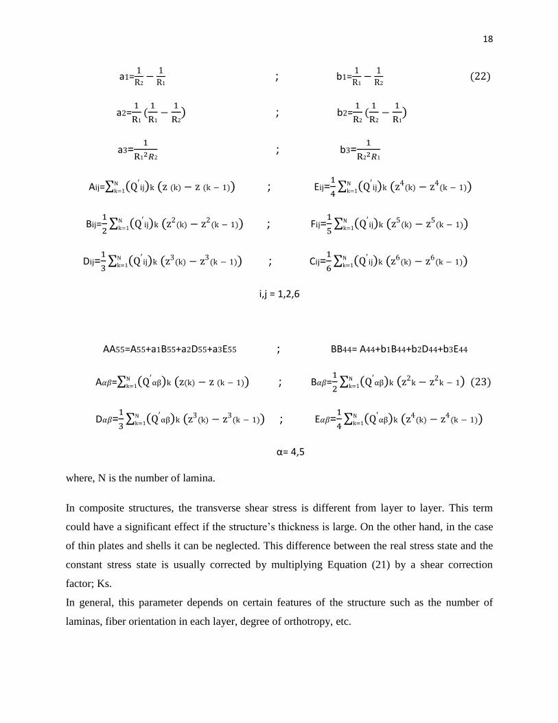
where, N is the number of lamina.

In composite structures, the transverse shear stress is different from layer to layer. This term

could have a significant effect if the structure‘s thickness is large. On the other hand, in the case

of thin plates and shells it can be neglected. This difference between the real stress state and the

constant stress state is usually corrected by multiplying Equation (21) by a shear correction

factor; Ks.

In general, this parameter depends on certain features of the structure such as the number of

laminas, fiber orientation in each layer, degree of orthotropy, etc.

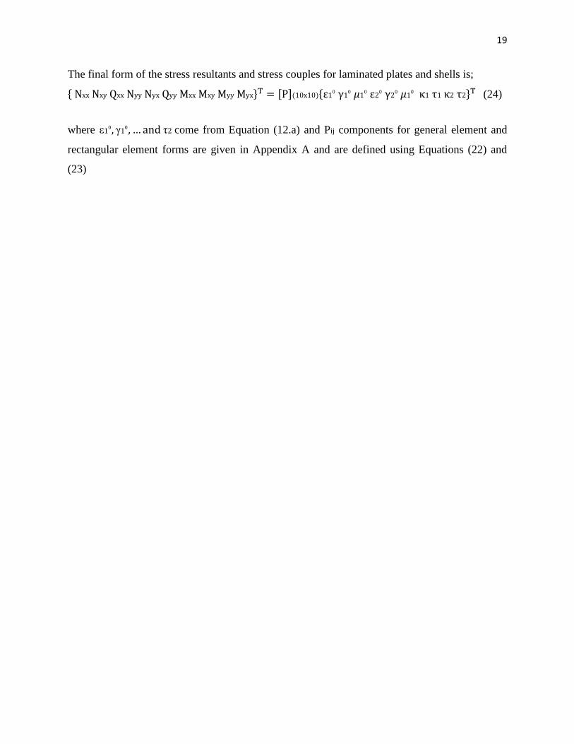
19

The final form of the stress resultants and stress couples for laminated plates and shells is;

{ } [ ] {

} (24)

where τ come from Equation (12.a) and Pij components for general element and

rectangular element forms are given in Appendix A and are defined using Equations (22) and

(23)

20

CHAPTER 3 SOLID FINITE ELEMENT MODEL

3.1 Structure modeling

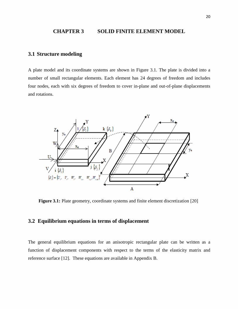
A plate model and its coordinate systems are shown in Figure 3.1. The plate is divided into a

number of small rectangular elements. Each element has 24 degrees of freedom and includes

four nodes, each with six degrees of freedom to cover in-plane and out-of-plane displacements

and rotations.

Figure 3.1: Plate geometry, coordinate systems and finite element discretization [20]

3.2 Equilibrium equations in terms of displacement

The general equilibrium equations for an anisotropic rectangular plate can be written as a

function of displacement components with respect to the terms of the elasticity matrix and

reference surface [12]. These equations are available in Appendix B.

21

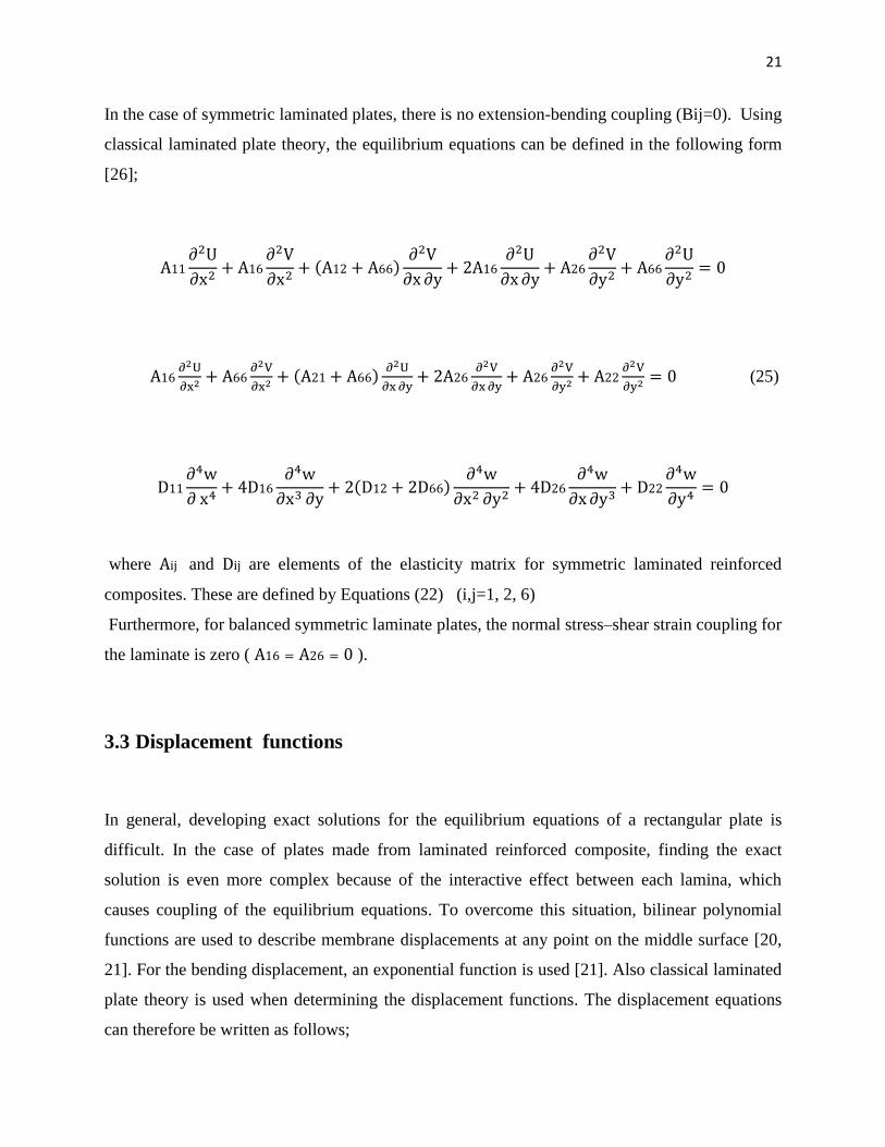
In the case of symmetric laminated plates, there is no extension-bending coupling (Bij=0). Using

classical laminated plate theory, the equilibrium equations can be defined in the following form

[26];

(25)

where and are elements of the elasticity matrix for symmetric laminated reinforced

composites. These are defined by Equations (22) (i,j=1, 2, 6)

Furthermore, for balanced symmetric laminate plates, the normal stress–shear strain coupling for

the laminate is zero ( ).

3.3 Displacement functions

In general, developing exact solutions for the equilibrium equations of a rectangular plate is

difficult. In the case of plates made from laminated reinforced composite, finding the exact

solution is even more complex because of the interactive effect between each lamina, which

causes coupling of the equilibrium equations. To overcome this situation, bilinear polynomial

functions are used to describe membrane displacements at any point on the middle surface [20,

21]. For the bending displacement, an exponential function is used [21]. Also classical laminated

plate theory is used when determining the displacement functions. The displacement equations

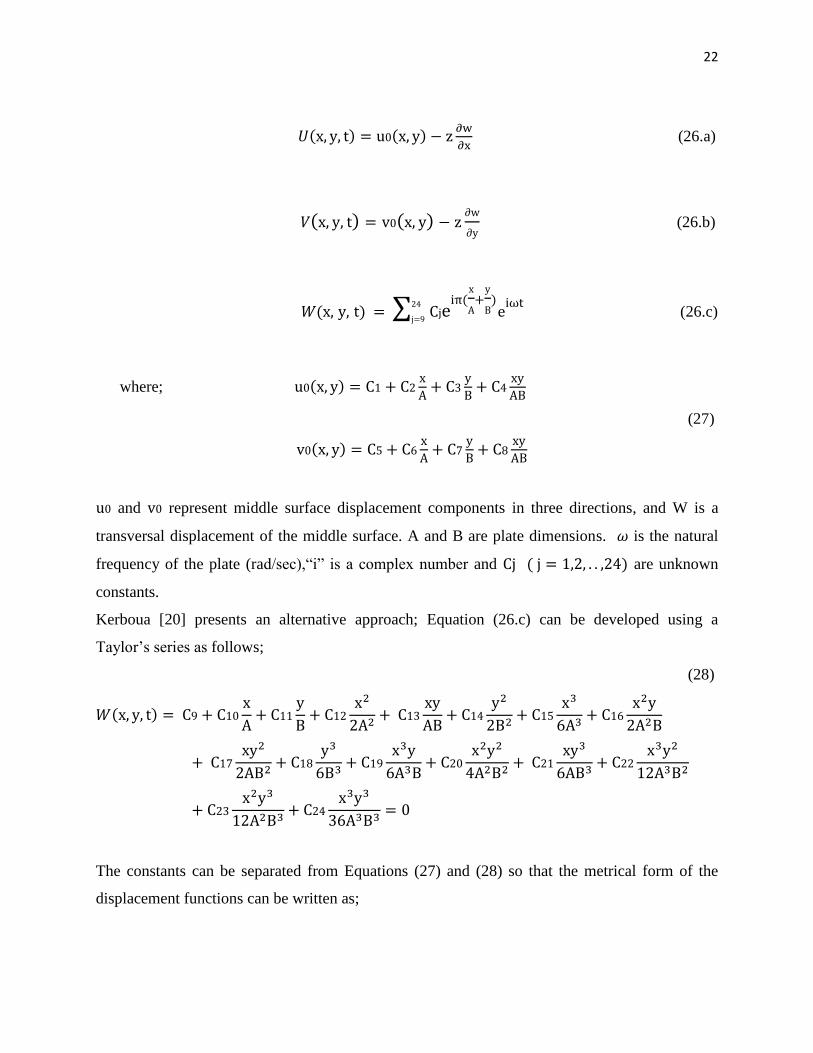
can therefore be written as follows;

22

(26.a)

(26.b)

∑

(26.c)

where;

(27)

and represent middle surface displacement components in three directions, and W is a

transversal displacement of the middle surface. A and B are plate dimensions. 𝜔 is the natural

frequency of the plate (rad/sec),―i‖ is a complex number and are unknown

constants.

Kerboua [20] presents an alternative approach; Equation (26.c) can be developed using a

Taylor‘s series as follows;

(28)

The constants can be separated from Equations (27) and (28) so that the metrical form of the

displacement functions can be written as;

23

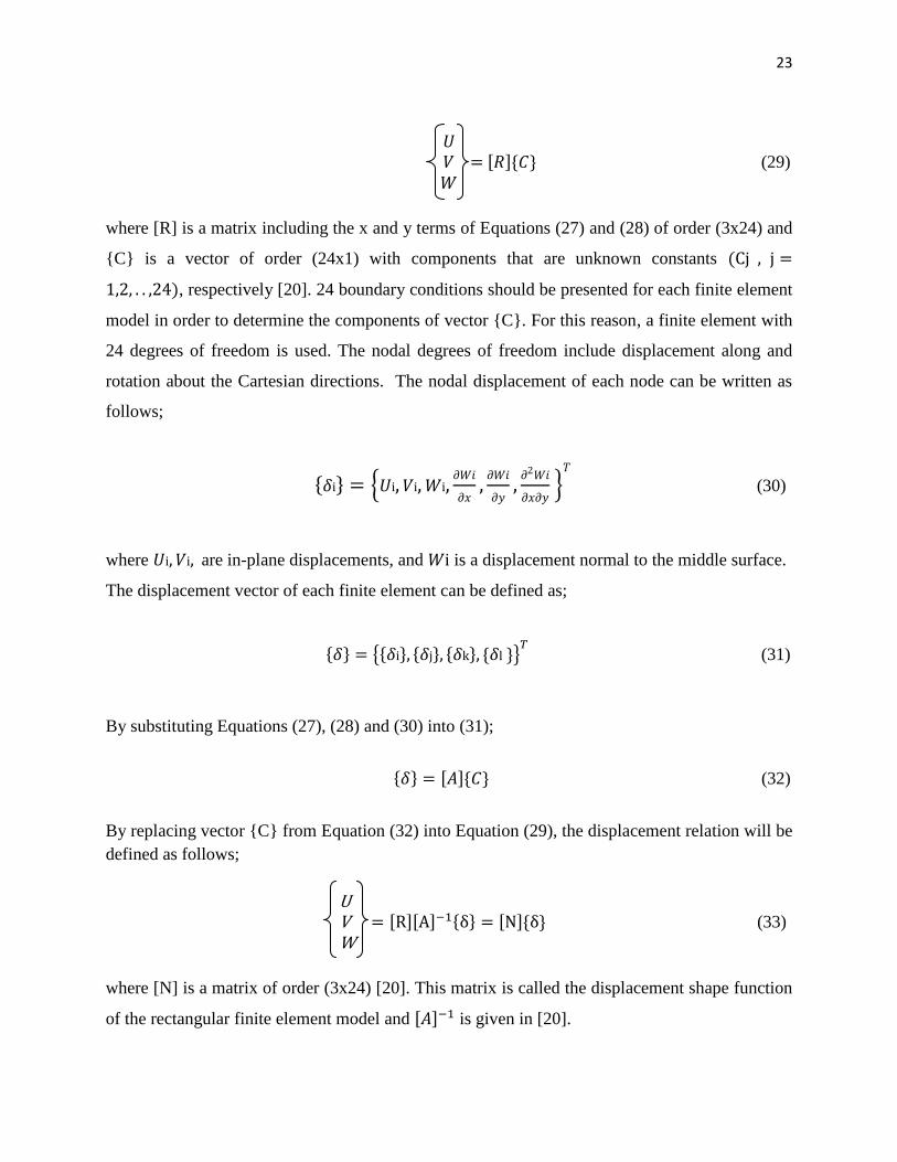
[ ]{ } (29)

where [R] is a matrix including the x and y terms of Equations (27) and (28) of order (3x24) and

{C} is a vector of order (24x1) with components that are unknown constants

, respectively [20]. 24 boundary conditions should be presented for each finite element

model in order to determine the components of vector {C}. For this reason, a finite element with

24 degrees of freedom is used. The nodal degrees of freedom include displacement along and

rotation about the Cartesian directions. The nodal displacement of each node can be written as

follows;

{ } ,

-

(30)

where are in-plane displacements, and is a displacement normal to the middle surface.

The displacement vector of each finite element can be defined as;

{ } {{ } { } { } { }} (31)

By substituting Equations (27), (28) and (30) into (31);

{ } [ ]{ } (32)

By replacing vector {C} from Equation (32) into Equation (29), the displacement relation will be

defined as follows;

U

V [ ][ ] { } [ ]{ } (33)

W

where [N] is a matrix of order (3x24) [20]. This matrix is called the displacement shape function

of the rectangular finite element model and [ ] is given in [20].

24

3.4 Linear strain-displacement relations

As previously explained in Section 2.2, the general relations for an anisotropic rectangular plate

are functions of in-plane and out-of-plane displacements. These are given in Appendix A. For a

laminated symmetry rectangular plate with respect to classical laminated plate theory, they are

given as[26];

(34)

where;

Equations (34) agree with those of classical homogeneous plate theory [26].

By substituting the displacement components of Equation (33) into Equation (34), the strain

vector can be obtained in terms of nodal displacements;

{ } [ ][ ] { } [ ]{ } (35)

where [ ] is a (6x24) matrix, given in [20].

3.5 Constitutive equations

As previously explained, the constitutive equations for a laminated rectangular plate without

taking into account the transverse shear deformations are defined as follows;

{ } [ ] { } (36)

25

where [ ] is the elasticity matrix for symmetric laminated reinforced composite plates (see

Appendix A). Depending on the material properties of the structure, symmetry or non-symmetry

of laminas and fiber orientation, some combination effects like bending-twisting, in-plane

extension-shear and extension-bending may exist in laminated composite plates and shells [27].

All of these couplings are defined by the components of [P].

By substituting the Equation (35) into (36), the stress-strain relations can be written as;

{ } [ ][ ]{ } (37)

Finally, the stiffness and mass matrices for one finite element can be given as;

[ ] ∫ ∫ [ ] [ ][ ]

(38)

[ ] ∫ ∫ [ ] [ ]

where is the plate thickness, is the density of the laminated plate, and are the

dimensions of the rectangular finite element and [P], [N] and [B] are as previously developed in

Equations (24), (33) and (35). By replacing them in Equation (38) we obtain;

[ ] [[ ] ] (∫ ∫ [ ] [ ][ ]

) [ ]

(39)

[ ] [[ ] ] (∫ ∫ [ ] [ ]

) [ ]

26

CHAPTER 4 DYNAMIC FLUID-STRUCTURE INTERACTIONS

In this chapter the effect of fluid on plate is going to study. Also several boundary conditions will

applied to the models then mass, stiffness and damping matrices for fluid will develop. Finally,

the eigenvalue solution will explain.

4.1 Assumptions

In this work, it is assumed that the structure is subjected to potential fluid flow and the effect of

this interaction is the dynamic fluid pressure applied to the structure. Fluid pressure can be

represented as a function of out-of-plane displacement, and it also induces inertial, Coriolis and

centrifugal forces. The assumptions below are taken into account in our mathematical model;

The fluid flow is a potential

The fluid is incompressible

The fluid is inviscid

The deformations are small (linear vibration)

The distribution of Fluid flow velocity is constant across the plate section

4.2 Equation of motion

By combining fluid and solid global matrices, the equations of motion of a plate subjected to a

fluid can be expressed as follows; [13]

([[ ] [ ]]){ ̈ } [ ] [ ] { ̇} [ ] [ ] { } { } (40)

where ‗s‘ and ‗f‘ refer to the structure and fluid. [ ], [ ], [ ] are the global mass, damping

and stiffness of the laminated plate, [ ], [ ]and [ ] are the same as plate matrices for fluid

and express the inertial, Coriolis and centrifugal forces and { } is the external forces. Also, { }

represents the global displacement vector. In this model the coordinate systems for structure and

finite elements are parallel so there is no difference between the angle of local and global

coordinate systems, however in other situations this may not be the case [28].

27

4.3 Development of fluid matrices

Working with the assumptions outlined above, to determine mass, stiffness and damping

matrices for the fluid-structure system, the pressure induced on the plate by the fluid must be

defined. The first step to do so involves using the Laplace equation and ensuring that the

potential flow function is satisfied. In the Cartesian coordinate system this relation can be

represented as follows; [19]

Another approach for connecting the potential function , fluid pressure , fluid velocity

and fluid density is using the Bernoulli equation, expressed as:[20]

(

)

Z=0 (42) The fluid velocity components in , and directions in the Cartesian coordinate system can be

written as derivations of the potential function as follows;

(43)

where is the fluid velocity in the direction.

By substituting Equation (43) into (42) and considering just linear terms, the dynamic pressure

applied to the surface of the plate can be represented as follows;

[ (

)]

Z=0 (44)

28

To allow perfect contact between the plate surface and the tangential fluid layer, the

impermeability condition should be taken into account. In other words; ―The impermeability

condition of the structure surface requires that the out-of-plane velocity component of the fluid

on the plate surface should match the instantaneous rate of change of the plate displacement in

the transversal direction‖[20]

Z=0 (45)

If it is considered that the fluid has zero velocity , the equation above can be written as;

Z=0 or h (46)

The potential fluid , is a function of , , and . We can separate it into two different

functions;

(47) To define these unknown functions, introducing Equation (47) into (45); one can obtain:

[

⁄

]

z=0 (48)

Then substituting Equation (48) into (47) result in:

[

⁄

]

Z=0 (50)

29

In Equation (50) the only undefined function is . has been presented before in Equation

(26.c).

By introducing the function obtained from Equation (50) into the Laplace equation

(41) the following differential equation can be obtained;

where;

𝜆 √ ⁄⁄ (52)

Equation (51) is a homogeneous linear second-order differential equation, so its solution can be

represented as follows;

(53)

where and are unidentified constants. By introducing Equation (53) into (50), the potential

function takes the following form;

⁄

(54)

Now, two boundary conditions should be applied to the potential function in order to define the

unknown constants ( and ). The first boundary condition can be applied at the fluid-plate

interface ( ), where the impermeability condition should be satisfied. The second boundary

condition is finite and/or infinite fluid level on one or two sides of the plate (see Figures 4.1, 4.2

and 4.4).

30

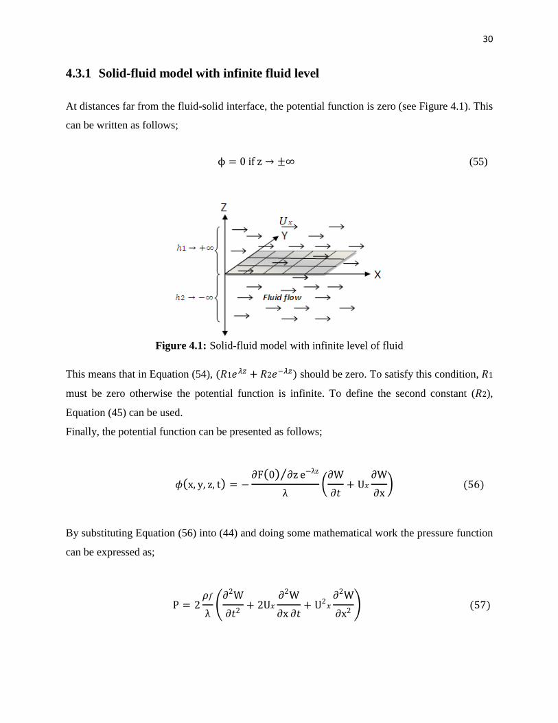
4.3.1 Solid-fluid model with infinite fluid level

At distances far from the fluid-solid interface, the potential function is zero (see Figure 4.1). This

can be written as follows;

(55)

Figure 4.1: Solid-fluid model with infinite level of fluid

This means that in Equation (54), should be zero. To satisfy this condition,

must be zero otherwise the potential function is infinite. To define the second constant ( ),

Equation (45) can be used.

Finally, the potential function can be presented as follows;

⁄

(

)

By substituting Equation (56) into (44) and doing some mathematical work the pressure function

can be expressed as;

.

/

31

If the plate is subjected to fluid on one side only, the induced fluid pressure is applied to one side

of plate, so Equation (57) should be divided by 2.

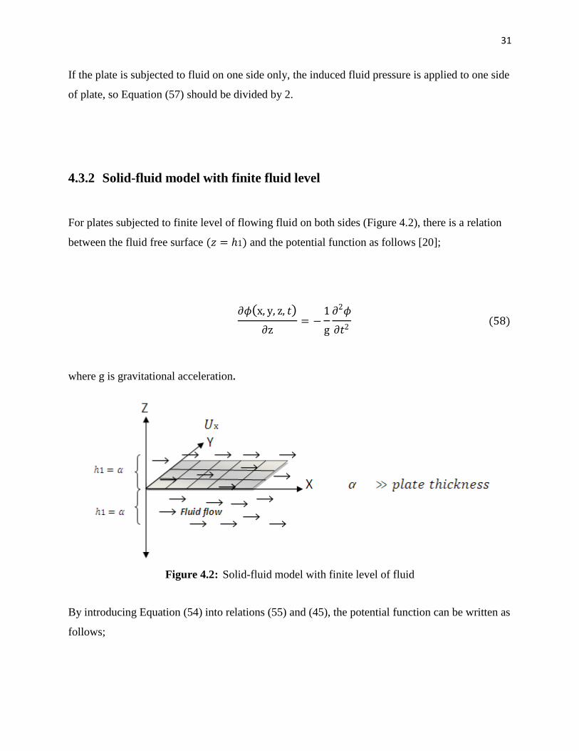
4.3.2 Solid-fluid model with finite fluid level

For plates subjected to finite level of flowing fluid on both sides (Figure 4.2), there is a relation

between the fluid free surface and the potential function as follows [20];

where is gravitational acceleration.

Figure 4.2: Solid-fluid model with finite level of fluid

By introducing Equation (54) into relations (55) and (45), the potential function can be written as

follows;

32

.

/ (

)

As Kerboua [20] shows, the constant trends to -1.

Finally, the dynamic pressure applied on both sides of the plate can be written as follows;[20]

.

/.

/

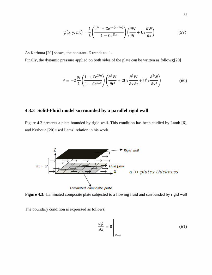
4.3.3 Solid-Fluid model surrounded by a parallel rigid wall

Figure 4.3 presents a plate bounded by rigid wall. This condition has been studied by Lamb [6],

and Kerboua [20] used Lams‘ relation in his work.

Figure 4.3: Laminated composite plate subjected to a flowing fluid and surrounded by rigid wall

The boundary condition is expressed as follows;

Z

33

To find the potential function, the same approach is used as presented in the previous section.

The potential function is written as follows; [20]

.

/(

)

And the induced fluid pressure is; [20]

.

/.

/

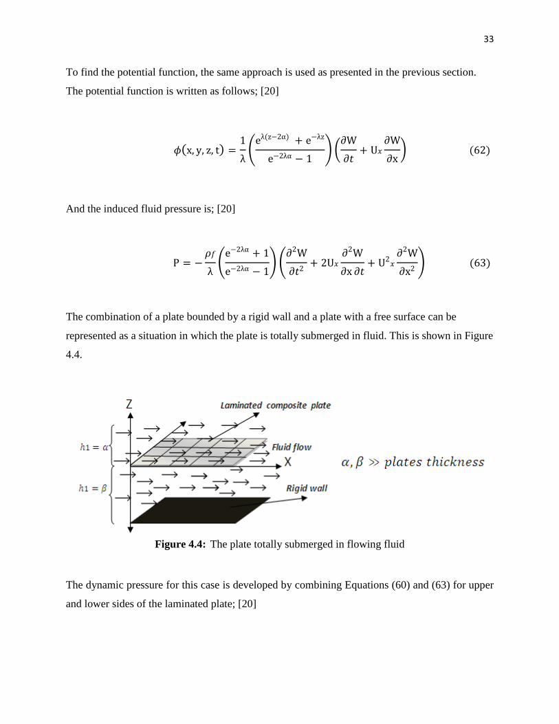
The combination of a plate bounded by a rigid wall and a plate with a free surface can be

represented as a situation in which the plate is totally submerged in fluid. This is shown in Figure

4.4.

Figure 4.4: The plate totally submerged in flowing fluid

The dynamic pressure for this case is developed by combining Equations (60) and (63) for upper

and lower sides of the laminated plate; [20]

34

.

/.

/

where α and 𝛽 are fluid levels above and below the plate. For a plate with a free surface (Figure

5.7 a) where 𝛼 the equation above will be written in the following form;

.

/.

/

4.3.4 Determination of force induced by fluid dynamic pressure

Using the finite element method, the fluid-induced force vector for an element of a plate can be

expressed as; [20]

{ } ∫ ∫ [ ] { }

where { } is a fluid-dynamic pressure vector. It describes the dynamic pressure applied on the

plate by the fluid. [ ] is a shape function matrix which is defined in Equation (33). The fluid

pressure is the only non-zero term of vector { } . So we have;

0

{ } 0 (67)

P

According to Equations (57), (60), (63), (64) and (65), the dynamic pressure can be written as a

function of the derivation of transverse displacement;

35

.

/

where;

𝜆 Infinite fluid level on both sides of the plate (Figure 4.1)

𝜆( 𝜆𝛼

𝜆𝛼) Finite fluid level (α) on both sides of the plate (Figure 4.2)

𝜆( 𝜆𝛼

𝜆𝛼 ) Plate bounded by a parallel rigid wall (Figure 4.3)

𝜆( 𝜆𝛼

𝜆𝛼

𝜆𝛽

𝜆𝛽 ) Plate submerged completely in fluid (Figure 4.4)

𝜆( 𝜆𝛽

𝜆𝛽 ) Plate with free surface (Figure 5.6 a)

By substituting the transverse displacement, Equation (26.c), into Equation (68) and performing

the derivations, Equation (68) can be written as;

.

(

)

/

Also for transverse displacement we can write the following relation;

0

0 [ ][ ] { } (70)

W

36

Where [ ] is given in [20].

Substituting Equation (70) into (69), the fluid-dynamic pressure vector becomes;

{ } [ ][ ] ({ ̈}

{ ̇}

(

)

{ })

By replacing [ ] from Equation (33) and substituting Equation (71) into Equation (66) the fluid-

induced force is expressed as follows;

{ }

(∫ ∫ [[ ] ] [ ] [ ][ ] { ̈}

∫ ∫ [[ ] ] [ ] [ ][ ] { ̇}

(

)

∫ ∫[[ ] ] [ ] [ ][ ] { }

)

As previously mentioned, fluid-induced force is composed of mass, stiffness and damping fluid

matrices which describe inertial, Coriolis and centrifugal effects.

Fluid matrices for a finite element can therefore be written as; [20]

[ ] ∫ ∫ [[ ] ] [ ] [ ][ ]

[ ]

∫ ∫ [[ ] ] [ ] [ ][ ]

37

[ ] (

)

∫ ∫ [[ ] ] [ ] [ ][ ]

4.4 Global matrices and eigenvalue solution

In Figure 3.1, a rectangular plate is divided into quadrilateral finite elements. The elements are

the same shape as the plate but on a smaller scale. Using the theoretical approach the mass and

stiffness matrices are developed for a structural element, and also the mass, stiffness and

damping matrices are obtained for a fluid element. By superimposing these matrices for each

individual finite element we can obtain the global matrices used in Equation (40).

Following this, boundary conditions should be applied to the structure to reduce the size of

global matrices as per the following relation;

Where N is the number of nodes in the plate and NC is the number of constraints applied.

To solve Equation (40) and allow analysis of the free vibration of the system the equation

reduction technique can be used, as was previously done by Toorani [27] and Kerboua [19].

For the free vibration of the system, Equation (40) can be written in the following form;

*[ ] [ ]

[ ] [ ]+ {

{ ̈}

{ ̇}} *

[ ] [ ]

[ ] [ ]+ {

{ }̇

{ }} (75)

where;

[ ] [ ] [ ] [ ] [ ] [ ] [ ] [ ]

38

{ } is the global displacement vector. In this investigation the damping effect of the structure is

neglected ([ ] ). The eigenvalue problem is given by;

|[ZZ] [ ]|

where;

[ZZ] [[ ] [ ]

[ ] [ ] [ ] [ ]]

⁄ (77)

[ ] is the identity matrix, and is a natural frequency of system (rad/sec).

39

CHAPTER 5 RESULTS AND DISCUSSIONS

In this chapter the results of present method are compared with other methods for different cases.

The effect of boundary conditions and stacking sequence of laminas on natural frequency of

plates are studied. Finally the stability and instability situation of plates subjected to flowing

fluid is discussed.

5.1 Modal analysis of a laminated plate

5.1.1 Essential number of elements for accurate results

The accuracy of the finite element method strongly depends on the number of elements used to

discretize the model. For this reason, the first results are used to determine the essential number

of elements for accurate determination of the natural frequencies.

For this test, a plate was totally clamped on all sides. The material type and geometrical

properties used are as follows;

A 16-layer symmetric laminated graphite/epoxy rectangular plate with staking sequence: [45°, -

45°, O°, -45°, 45°, -45°, O°, 45°]sym, longitudinal modulus E1=173 GPa, transverse modulus

E2=7.2 GPa, Major Poisson‘s ratio ν12=0.29, Minor Poisson‘s ratio ν21=0.01, In-plane shear

modulus G12=G21=3.76 GPa and thickness h=2.72 mm. The plate dimensions are A=0.45 m and

B=0.3 m, material density ρ=1540 kg/ .

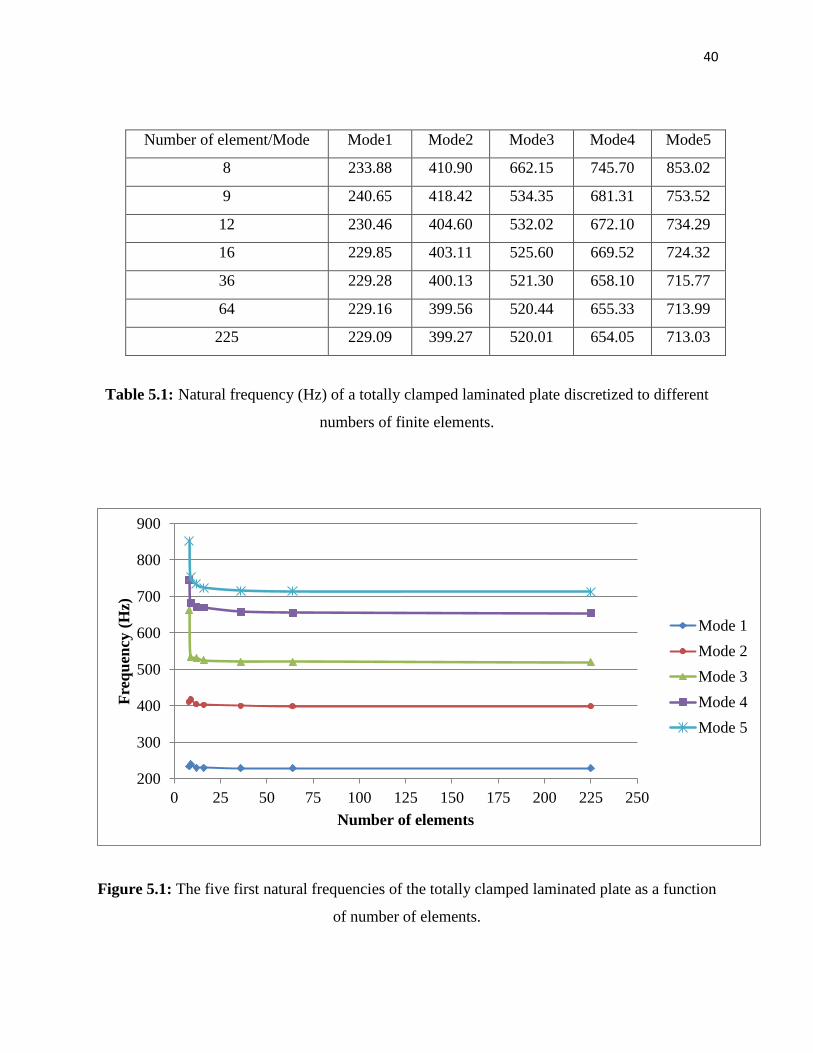
Table 5.1 shows the computed natural frequencies (Hz) of the model for the first five modes,

which have different numbers of elements. Also, in Figure 5.1, the relationship between the

frequencies and the number of finite elements is plotted for the first five modes. This graph

demonstrates the minimum number of elements required to achieve convergence on the natural

frequencies for both high and low levels.

As Figure 5.1 demonstrates, 16 elements are sufficient for the first three modes, but for higher

modes 36 elements are required to obtain fast convergence. Incidentally, for all of following

examples 64 elements are used in order to guarantee that the results will not be dependent on the

number of elements.

40

Number of element/Mode Mode1 Mode2 Mode3 Mode4 Mode5

8 233.88 410.90 662.15 745.70 853.02

9 240.65 418.42 534.35 681.31 753.52

12 230.46 404.60 532.02 672.10 734.29

16 229.85 403.11 525.60 669.52 724.32

36 229.28 400.13 521.30 658.10 715.77

64 229.16 399.56 520.44 655.33 713.99

225 229.09 399.27 520.01 654.05 713.03

Table 5.1: Natural frequency (Hz) of a totally clamped laminated plate discretized to different

numbers of finite elements.

Figure 5.1: The five first natural frequencies of the totally clamped laminated plate as a function

of number of elements.

200

300

400

500

600

700

800

900

0 25 50 75 100 125 150 175 200 225 250

Fre

qu

ency

(H

z)

Number of elements

Mode 1

Mode 2

Mode 3

Mode 4

Mode 5

41

5.1.2 Comparison of the present method with other investigations and

commercial software results

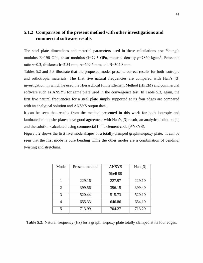
The steel plate dimensions and material parameters used in these calculations are: Young‘s

modulus E=196 GPa, shear modulus G=79.3 GPa, material density ρ=7860 kg/ , Poisson‗s

ratio ν=0.3, thickness h=2.54 mm, A=609.6 mm, and B=304.8 mm.

Tables 5.2 and 5.3 illustrate that the proposed model presents correct results for both isotropic

and orthotropic materials. The first five natural frequencies are compared with Han‘s [3]

investigation, in which he used the Hierarchical Finite Element Method (HFEM) and commercial

software such as ANSYS for same plate used in the convergence test. In Table 5.3, again, the

first five natural frequencies for a steel plate simply supported at its four edges are compared

with an analytical solution and ANSYS output data.

It can be seen that results from the method presented in this work for both isotropic and

laminated composite plates have good agreement with Han‘s [3] result, an analytical solution [1]

and the solution calculated using commercial finite element code (ANSYS).

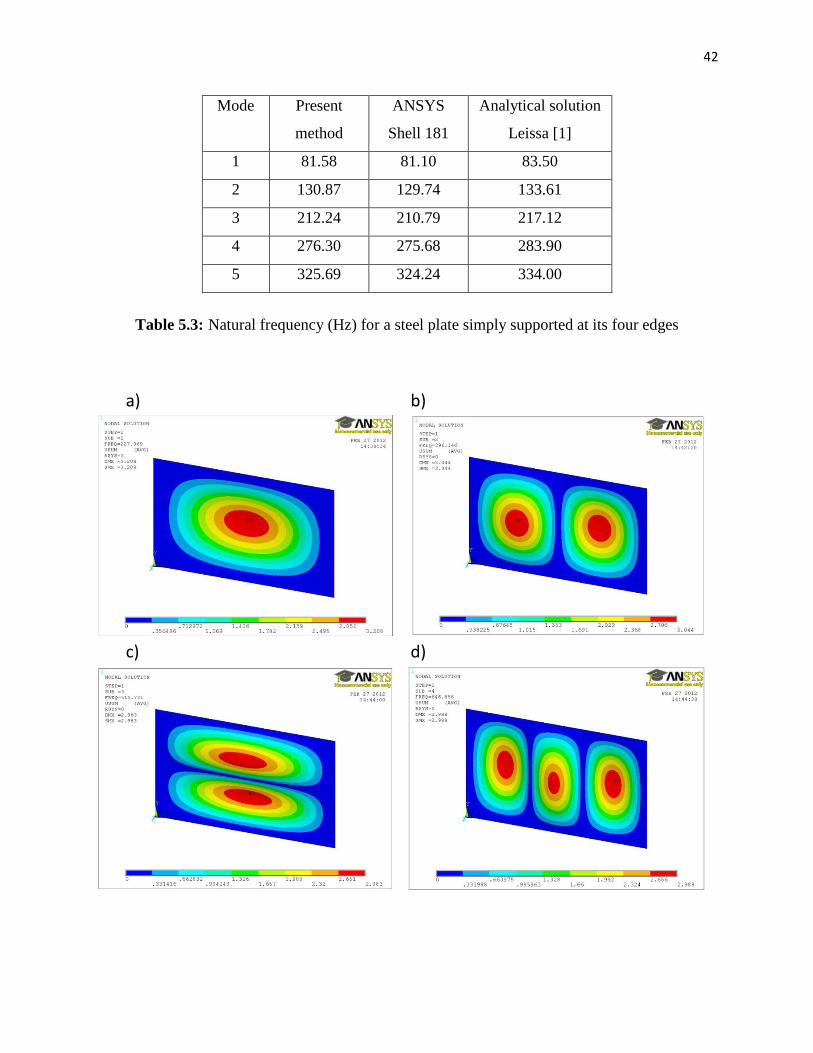
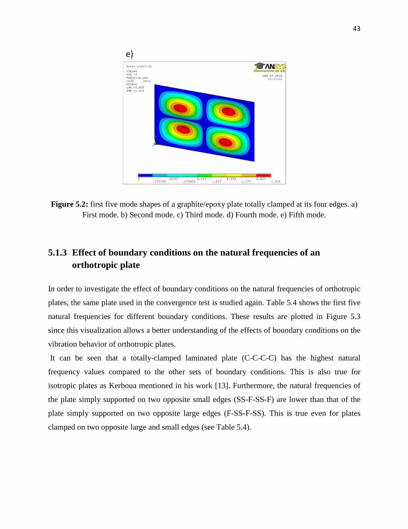
Figure 5.2 shows the first five mode shapes of a totally-clamped graphite/epoxy plate. It can be

seen that the first mode is pure bending while the other modes are a combination of bending,

twisting and stretching.

Mode Present method ANSYS

Shell 99

Han [3]

1 229.16 227.97 229.10

2 399.56 396.15 399.40

3 520.44 515.73 520.10

4 655.33 646.86 654.10

5 713.99 704.27 713.20

Table 5.2: Natural frequency (Hz) for a graphite/epoxy plate totally clamped at its four edges.

42

Mode Present

method

ANSYS

Shell 181

Analytical solution

Leissa [1]

1 81.58 81.10 83.50

2 130.87 129.74 133.61

3 212.24 210.79 217.12

4 276.30 275.68 283.90

5 325.69 324.24 334.00

Table 5.3: Natural frequency (Hz) for a steel plate simply supported at its four edges

a) b)

c) d)

43

e)

Figure 5.2: first five mode shapes of a graphite/epoxy plate totally clamped at its four edges. a)

First mode. b) Second mode. c) Third mode. d) Fourth mode. e) Fifth mode.

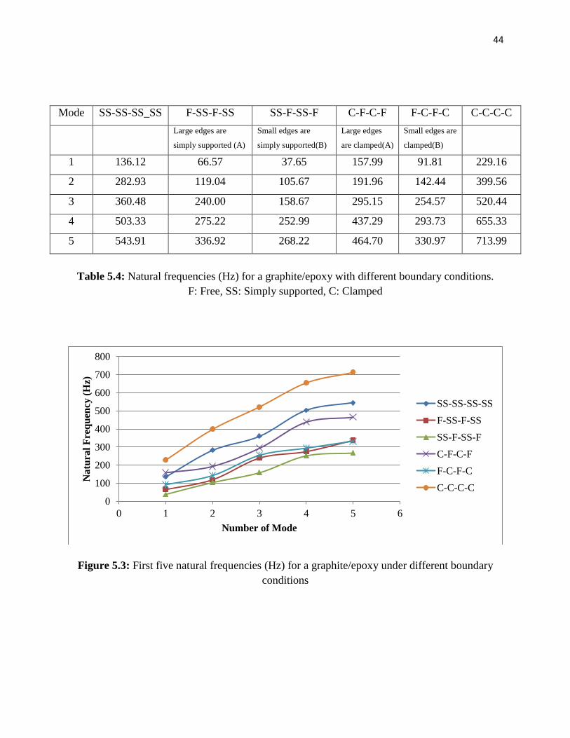
5.1.3 Effect of boundary conditions on the natural frequencies of an

orthotropic plate

In order to investigate the effect of boundary conditions on the natural frequencies of orthotropic

plates, the same plate used in the convergence test is studied again. Table 5.4 shows the first five

natural frequencies for different boundary conditions. These results are plotted in Figure 5.3

since this visualization allows a better understanding of the effects of boundary conditions on the

vibration behavior of orthotropic plates.

It can be seen that a totally-clamped laminated plate (C-C-C-C) has the highest natural

frequency values compared to the other sets of boundary conditions. This is also true for

isotropic plates as Kerboua mentioned in his work [13]. Furthermore, the natural frequencies of

the plate simply supported on two opposite small edges (SS-F-SS-F) are lower than that of the

plate simply supported on two opposite large edges (F-SS-F-SS). This is true even for plates

clamped on two opposite large and small edges (see Table 5.4).

44

Mode SS-SS-SS_SS F-SS-F-SS SS-F-SS-F C-F-C-F F-C-F-C C-C-C-C

Large edges are

simply supported (A)

Small edges are

simply supported(B) Large edges

are clamped(A) Small edges are

clamped(B)

1 136.12 66.57 37.65 157.99 91.81 229.16

2 282.93 119.04 105.67 191.96 142.44 399.56

3 360.48 240.00 158.67 295.15 254.57 520.44

4 503.33 275.22 252.99 437.29 293.73 655.33

5 543.91 336.92 268.22 464.70 330.97 713.99

Table 5.4: Natural frequencies (Hz) for a graphite/epoxy with different boundary conditions.

F: Free, SS: Simply supported, C: Clamped

Figure 5.3: First five natural frequencies (Hz) for a graphite/epoxy under different boundary

conditions

0

100

200

300

400

500

600

700

800

0 1 2 3 4 5 6

Natu

ral

Fre

qu

ency

(H

z)

Number of Mode

SS-SS-SS-SS

F-SS-F-SS

SS-F-SS-F

C-F-C-F

F-C-F-C

C-C-C-C

45

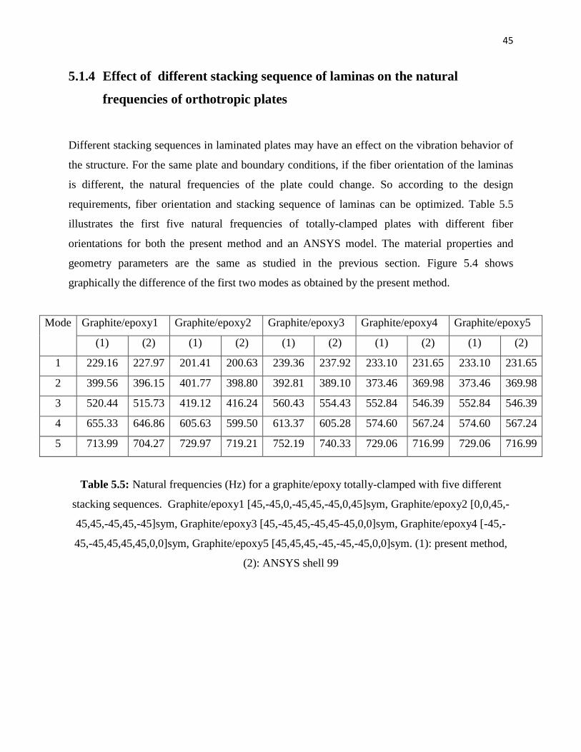
5.1.4 Effect of different stacking sequence of laminas on the natural

frequencies of orthotropic plates

Different stacking sequences in laminated plates may have an effect on the vibration behavior of

the structure. For the same plate and boundary conditions, if the fiber orientation of the laminas

is different, the natural frequencies of the plate could change. So according to the design

requirements, fiber orientation and stacking sequence of laminas can be optimized. Table 5.5

illustrates the first five natural frequencies of totally-clamped plates with different fiber

orientations for both the present method and an ANSYS model. The material properties and

geometry parameters are the same as studied in the previous section. Figure 5.4 shows

graphically the difference of the first two modes as obtained by the present method.

Mode Graphite/epoxy1 Graphite/epoxy2 Graphite/epoxy3 Graphite/epoxy4 Graphite/epoxy5

(1) (2) (1) (2) (1) (2) (1) (2) (1) (2)

1 229.16 227.97 201.41 200.63 239.36 237.92 233.10 231.65 233.10 231.65

2 399.56 396.15 401.77 398.80 392.81 389.10 373.46 369.98 373.46 369.98

3 520.44 515.73 419.12 416.24 560.43 554.43 552.84 546.39 552.84 546.39

4 655.33 646.86 605.63 599.50 613.37 605.28 574.60 567.24 574.60 567.24

5 713.99 704.27 729.97 719.21 752.19 740.33 729.06 716.99 729.06 716.99

Table 5.5: Natural frequencies (Hz) for a graphite/epoxy totally-clamped with five different

stacking sequences. Graphite/epoxy1 [45,-45,0,-45,45,-45,0,45]sym, Graphite/epoxy2 [0,0,45,-

45,45,-45,45,-45]sym, Graphite/epoxy3 [45,-45,45,-45,45-45,0,0]sym, Graphite/epoxy4 [-45,-

45,-45,45,45,45,0,0]sym, Graphite/epoxy5 [45,45,45,-45,-45,-45,0,0]sym. (1): present method,

(2): ANSYS shell 99

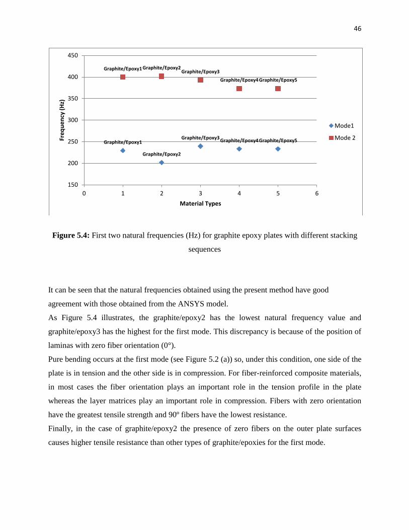
46

Figure 5.4: First two natural frequencies (Hz) for graphite epoxy plates with different stacking

sequences

It can be seen that the natural frequencies obtained using the present method have good

agreement with those obtained from the ANSYS model.

As Figure 5.4 illustrates, the graphite/epoxy2 has the lowest natural frequency value and

graphite/epoxy3 has the highest for the first mode. This discrepancy is because of the position of

laminas with zero fiber orientation (0°).

Pure bending occurs at the first mode (see Figure 5.2 (a)) so, under this condition, one side of the

plate is in tension and the other side is in compression. For fiber-reinforced composite materials,

in most cases the fiber orientation plays an important role in the tension profile in the plate

whereas the layer matrices play an important role in compression. Fibers with zero orientation

have the greatest tensile strength and 90º fibers have the lowest resistance.

Finally, in the case of graphite/epoxy2 the presence of zero fibers on the outer plate surfaces

causes higher tensile resistance than other types of graphite/epoxies for the first mode.

Graphite/Epoxy1

Graphite/Epoxy2

Graphite/Epoxy3 Graphite/Epoxy4 Graphite/Epoxy5

Graphite/Epoxy1 Graphite/Epoxy2 Graphite/Epoxy3

Graphite/Epoxy4 Graphite/Epoxy5

150

200

250

300

350

400

450

0 1 2 3 4 5 6

Fre

qu

en

cy (

Hz)

Material Types

Mode1

Mode 2

47

5.2 Modal analysis of a plate totally submerged in fluid

In this section, vibration analysis of a plate immersed in water and vacuo is studied. Both

isotropic and laminated plates are considered in following examples and the natural frequency of

plates with and without water are compared.

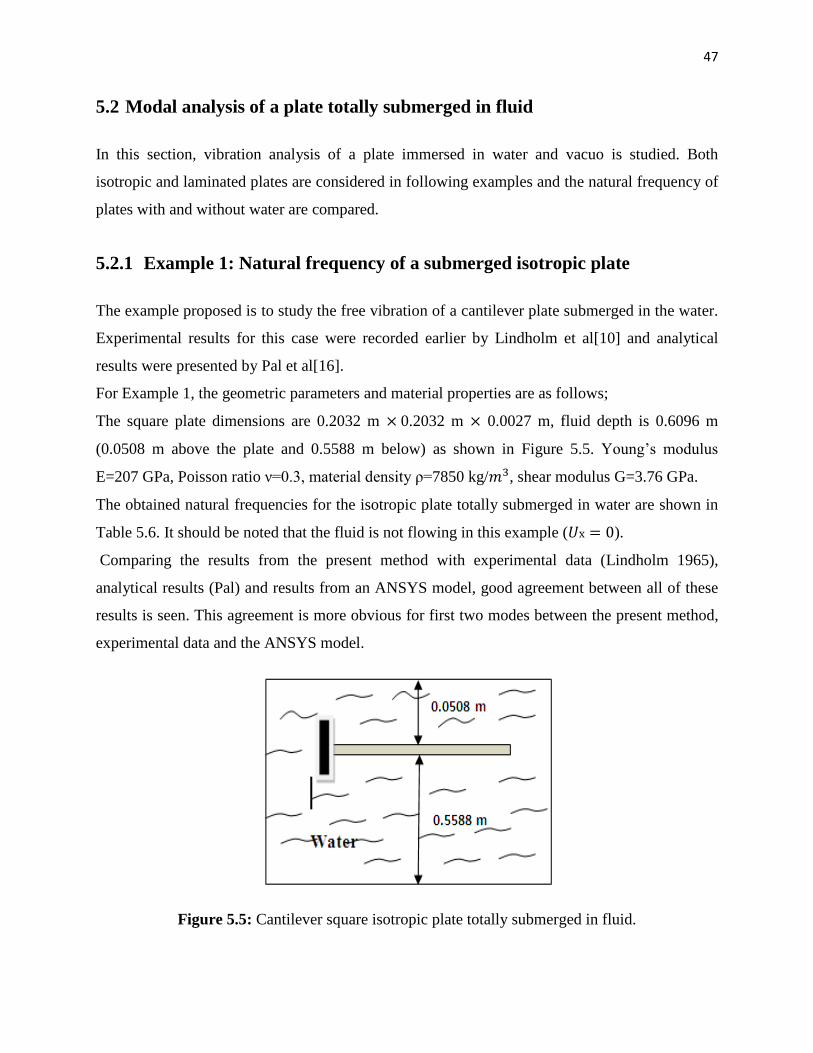
5.2.1 Example 1: Natural frequency of a submerged isotropic plate

The example proposed is to study the free vibration of a cantilever plate submerged in the water.

Experimental results for this case were recorded earlier by Lindholm et al[10] and analytical

results were presented by Pal et al[16].

For Example 1, the geometric parameters and material properties are as follows;

The square plate dimensions are 0.2032 m 0.2032 m 0.0027 m, fluid depth is 0.6096 m

(0.0508 m above the plate and 0.5588 m below) as shown in Figure 5.5. Young‘s modulus

E=207 GPa, Poisson ratio ν=0.3, material density ρ=7850 kg/ , shear modulus G=3.76 GPa.

The obtained natural frequencies for the isotropic plate totally submerged in water are shown in

Table 5.6. It should be noted that the fluid is not flowing in this example ( ).

Comparing the results from the present method with experimental data (Lindholm 1965),

analytical results (Pal) and results from an ANSYS model, good agreement between all of these

results is seen. This agreement is more obvious for first two modes between the present method,

experimental data and the ANSYS model.

Figure 5.5: Cantilever square isotropic plate totally submerged in fluid.

48

Mode Present method Lindholm Pal ANSYS Shell 181

1 24.90 23.30 24.50 24.11

2 61.04 67.80 74.30 58.98

3 152.74 158.00 179.70 147.91

4 195.14 234.00 262.80 188.80

5 222.16 267.00 287.90 214.67

Table 5.6: Frequencies (Hz) for an isotropic cantilever plate totally submerged in water.

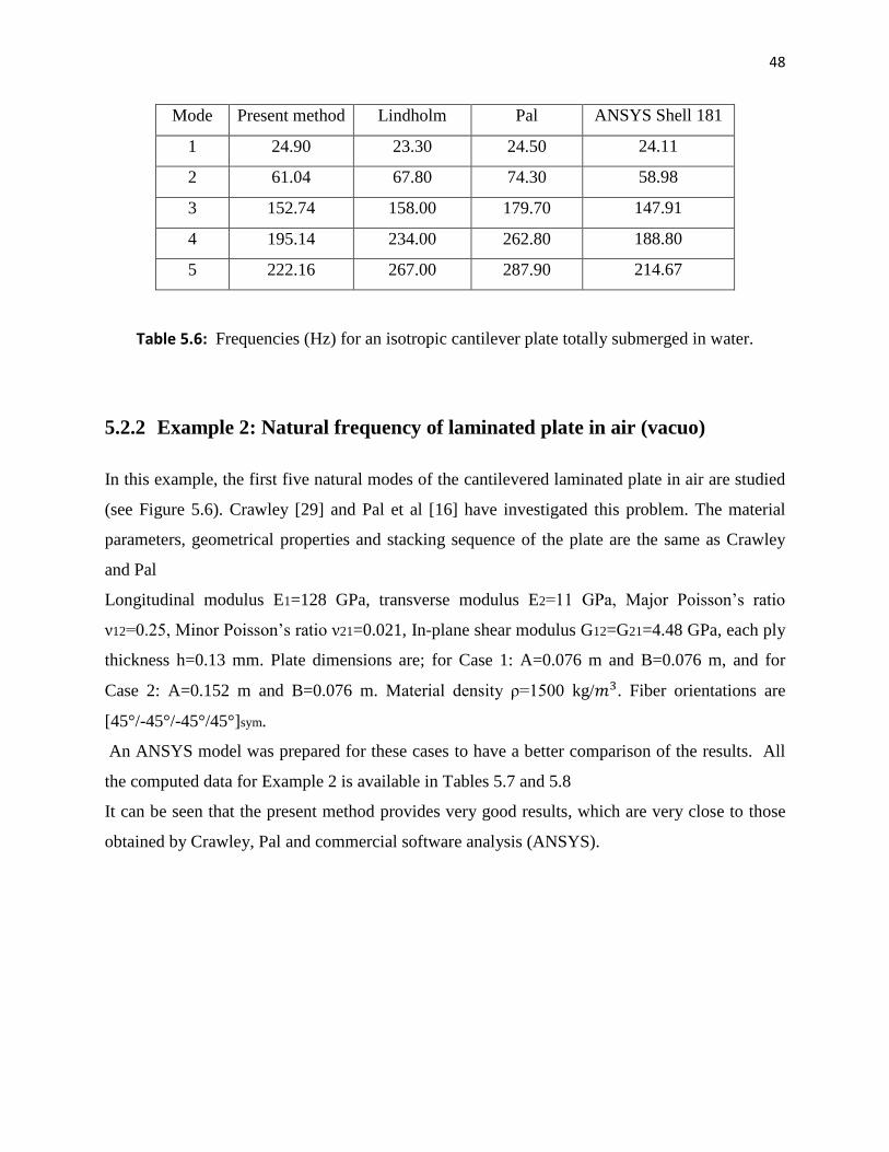
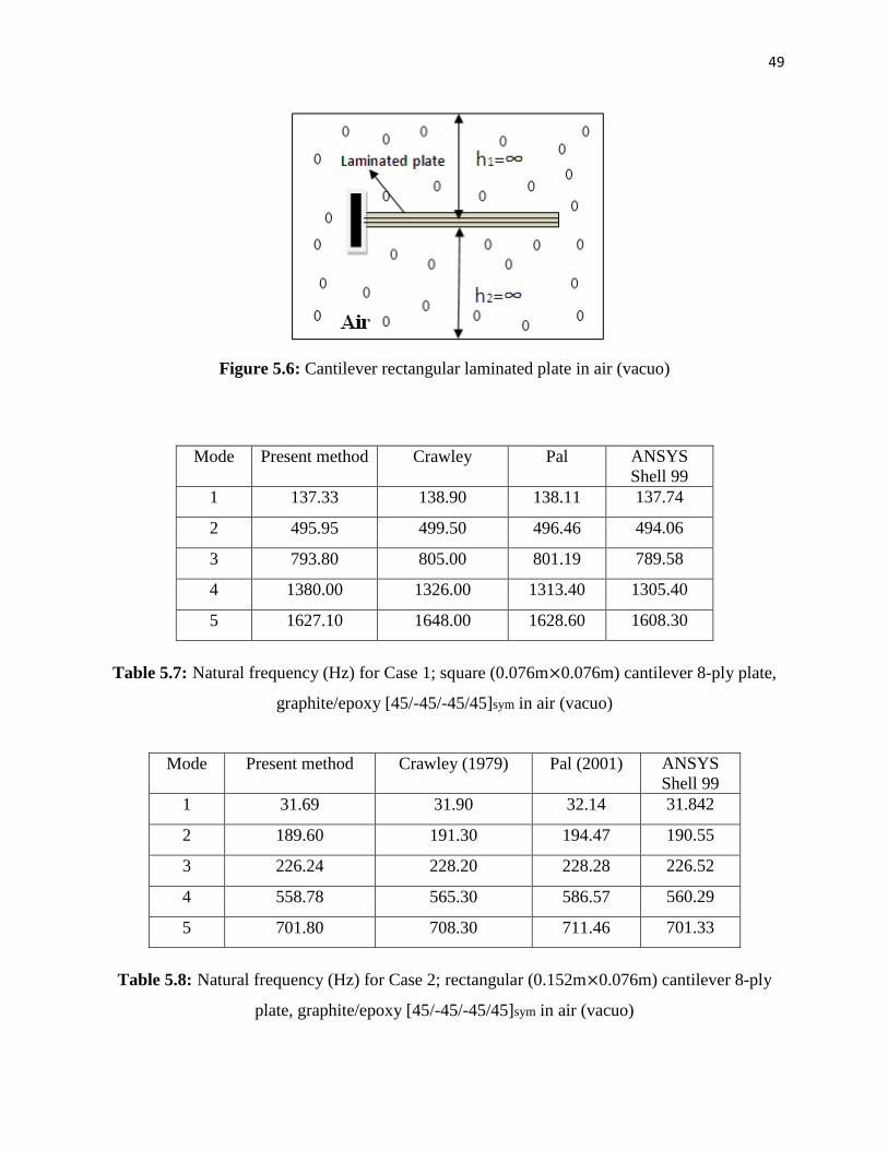
5.2.2 Example 2: Natural frequency of laminated plate in air (vacuo)

In this example, the first five natural modes of the cantilevered laminated plate in air are studied

(see Figure 5.6). Crawley [29] and Pal et al [16] have investigated this problem. The material

parameters, geometrical properties and stacking sequence of the plate are the same as Crawley

and Pal

Longitudinal modulus E1=128 GPa, transverse modulus E2=11 GPa, Major Poisson‘s ratio

ν12=0.25, Minor Poisson‘s ratio ν21=0.021, In-plane shear modulus G12=G21=4.48 GPa, each ply

thickness h=0.13 mm. Plate dimensions are; for Case 1: A=0.076 m and B=0.076 m, and for

Case 2: A=0.152 m and B=0.076 m. Material density ρ=1500 kg/ . Fiber orientations are

[45°/-45°/-45°/45°]sym.

An ANSYS model was prepared for these cases to have a better comparison of the results. All

the computed data for Example 2 is available in Tables 5.7 and 5.8

It can be seen that the present method provides very good results, which are very close to those

obtained by Crawley, Pal and commercial software analysis (ANSYS).

49

Figure 5.6: Cantilever rectangular laminated plate in air (vacuo)

Mode Present method Crawley Pal ANSYS

Shell 99

1 137.33 138.90 138.11 137.74

2 495.95 499.50 496.46 494.06

3 793.80 805.00 801.19 789.58

4 1380.00 1326.00 1313.40 1305.40

5 1627.10 1648.00 1628.60 1608.30

Table 5.7: Natural frequency (Hz) for Case 1; square (0.076m 0.076m) cantilever 8-ply plate,

graphite/epoxy [45/-45/-45/45]sym in air (vacuo)

Mode Present method Crawley (1979) Pal (2001) ANSYS

Shell 99

1 31.69 31.90 32.14 31.842

2 189.60 191.30 194.47 190.55

3 226.24 228.20 228.28 226.52

4 558.78 565.30 586.57 560.29

5 701.80 708.30 711.46 701.33

Table 5.8: Natural frequency (Hz) for Case 2; rectangular (0.152m 0.076m) cantilever 8-ply

plate, graphite/epoxy [45/-45/-45/45]sym in air (vacuo)

50

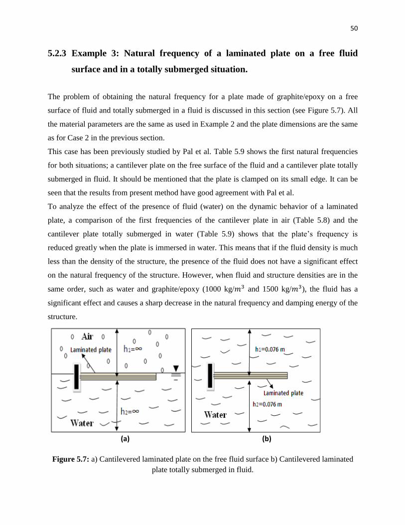
5.2.3 Example 3: Natural frequency of a laminated plate on a free fluid

surface and in a totally submerged situation.

The problem of obtaining the natural frequency for a plate made of graphite/epoxy on a free

surface of fluid and totally submerged in a fluid is discussed in this section (see Figure 5.7). All

the material parameters are the same as used in Example 2 and the plate dimensions are the same

as for Case 2 in the previous section.

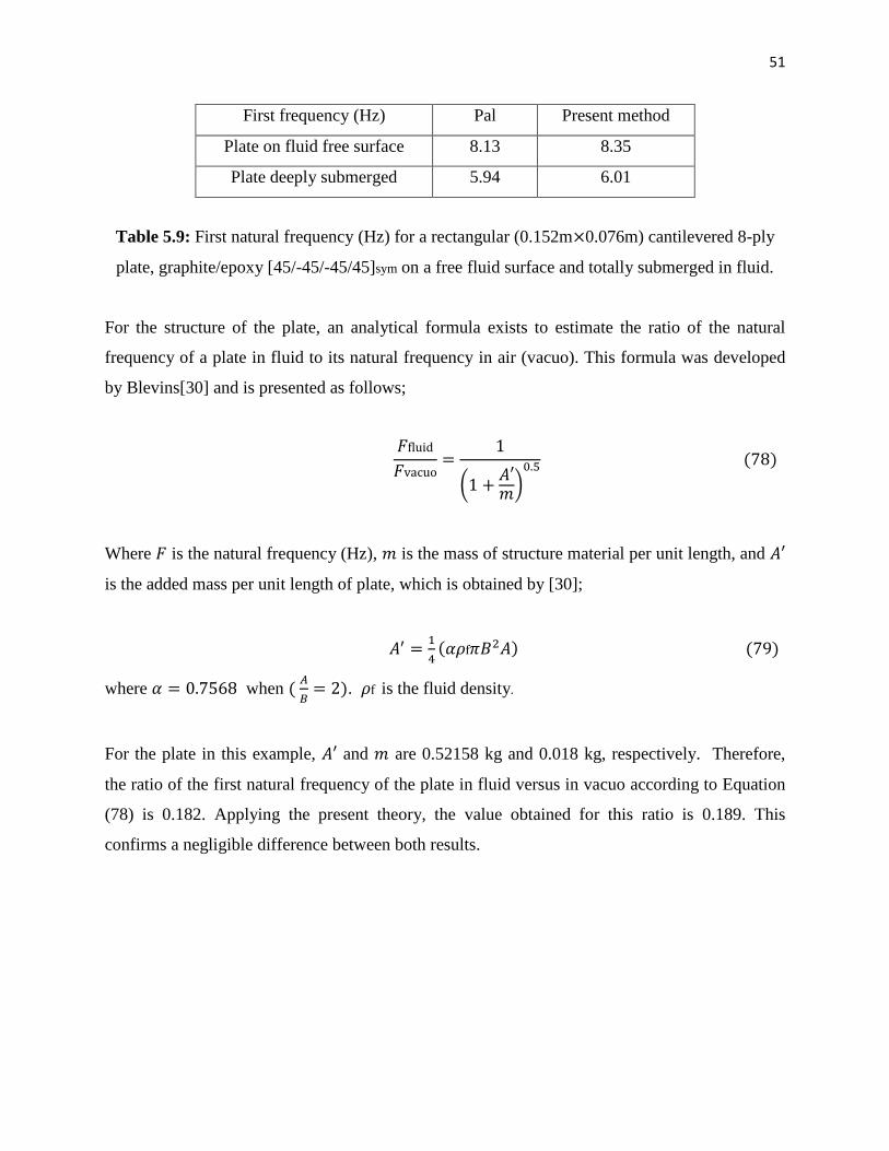
This case has been previously studied by Pal et al. Table 5.9 shows the first natural frequencies

for both situations; a cantilever plate on the free surface of the fluid and a cantilever plate totally

submerged in fluid. It should be mentioned that the plate is clamped on its small edge. It can be

seen that the results from present method have good agreement with Pal et al.

To analyze the effect of the presence of fluid (water) on the dynamic behavior of a laminated

plate, a comparison of the first frequencies of the cantilever plate in air (Table 5.8) and the

cantilever plate totally submerged in water (Table 5.9) shows that the plate‘s frequency is

reduced greatly when the plate is immersed in water. This means that if the fluid density is much

less than the density of the structure, the presence of the fluid does not have a significant effect

on the natural frequency of the structure. However, when fluid and structure densities are in the

same order, such as water and graphite/epoxy (1000 kg/ and 1500 kg/ ), the fluid has a

significant effect and causes a sharp decrease in the natural frequency and damping energy of the

structure.

(a) (b)

Figure 5.7: a) Cantilevered laminated plate on the free fluid surface b) Cantilevered laminated

plate totally submerged in fluid.

51

First frequency (Hz) Pal Present method

Plate on fluid free surface 8.13 8.35

Plate deeply submerged 5.94 6.01

Table 5.9: First natural frequency (Hz) for a rectangular (0.152m 0.076m) cantilevered 8-ply

plate, graphite/epoxy [45/-45/-45/45]sym on a free fluid surface and totally submerged in fluid.

For the structure of the plate, an analytical formula exists to estimate the ratio of the natural

frequency of a plate in fluid to its natural frequency in air (vacuo). This formula was developed

by Blevins[30] and is presented as follows;

( )

Where is the natural frequency (Hz), is the mass of structure material per unit length, and

is the added mass per unit length of plate, which is obtained by [30];

𝛼 (79)

where 𝛼 when

. is the fluid density.

For the plate in this example, and are 0.52158 kg and 0.018 kg, respectively. Therefore,

the ratio of the first natural frequency of the plate in fluid versus in vacuo according to Equation

(78) is 0.182. Applying the present theory, the value obtained for this ratio is 0.189. This

confirms a negligible difference between both results.

52

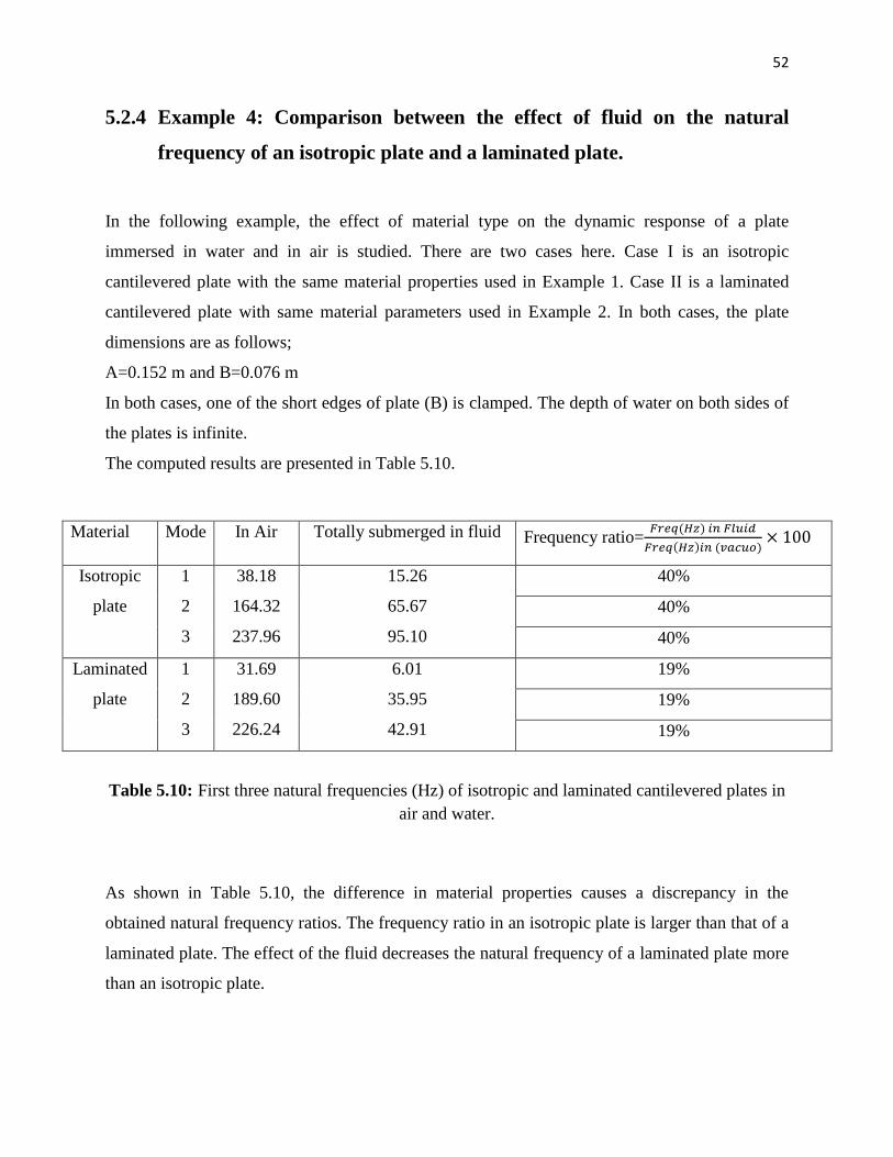
5.2.4 Example 4: Comparison between the effect of fluid on the natural

frequency of an isotropic plate and a laminated plate.

In the following example, the effect of material type on the dynamic response of a plate

immersed in water and in air is studied. There are two cases here. Case І is an isotropic

cantilevered plate with the same material properties used in Example 1. Case ІІ is a laminated

cantilevered plate with same material parameters used in Example 2. In both cases, the plate

dimensions are as follows;

A=0.152 m and B=0.076 m

In both cases, one of the short edges of plate (B) is clamped. The depth of water on both sides of

the plates is infinite.

The computed results are presented in Table 5.10.

Material Mode In Air Totally submerged in fluid Frequency ratio=

Isotropic

plate

1

2

3

38.18

164.32

237.96

15.26

65.67

95.10

40%

40%

40%

Laminated

plate

1

2

3

31.69

189.60

226.24

6.01

35.95

42.91

19%

19%

19%

Table 5.10: First three natural frequencies (Hz) of isotropic and laminated cantilevered plates in

air and water.

As shown in Table 5.10, the difference in material properties causes a discrepancy in the

obtained natural frequency ratios. The frequency ratio in an isotropic plate is larger than that of a

laminated plate. The effect of the fluid decreases the natural frequency of a laminated plate more

than an isotropic plate.

53

5.3 Stability analysis of a plate subjected to flowing fluid

The dynamic response and natural frequency of structures change with fluid velocity. Flowing

fluid can cause structural instability. Instability caused by the influence of fluid flow is a vast

subject because it varies depending on the fluid type and fluid speed. For an incompressible fluid

such as water, most of the research in this area focuses on low flowing fluid rates, called

‗subsonic flow‘. These can cause static aero-elastic instability or ‗divergence‘. On the other

hand, for compressive fluids such as air one can reach very high flowing fluid rates, called

‗supersonic flow‘ and ‗hypersonic flow‘. These high flow rates can cause dynamic aero-elastic

instability, known as ‗Flutter‘.

In a physical plate system, it is expected that divergence will cause large plate deflections. This

expectation is different for flutter however. Once the system dynamic pressure reaches a level for

flutter to occur, the movement of the plate creates significant pressure fluctuations, which

modify the plate motion.

Generally, increasing the rate of fluid causes an increased probability of structure instability.

In this work we investigate the static instability of isotropic and laminated plates. The effect of

stacking sequence on critical velocity is also discussed.

5.3.1 Example 1: Laminated plate clamped on two opposite edges coupled

with flowing fluid

In this example, the plate used in section 5.1.1 (Graphite/epoxy1), is subjected to flowing fluid.

The plate is clamped on its two small opposite edges (see Figure 5.8). The trend of changes of

the first three natural frequencies versus increasing fluid flow rate is shown in Figure 5.9.

Essentially, increasing the fluid flow rate causes an increase in dynamic pressure and

consequently the vibrating frequencies of the plate decrease. Mathematically, static instability

occurs when the frequency values change from positive to negative. At this point, the fluid

velocity reaches its critical value. It is very important that this point is well defined when

designing structures coupled with flowing fluid.

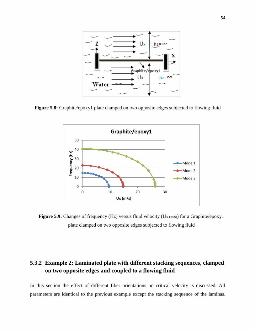
54

Figure 5.8: Graphite/epoxy1 plate clamped on two opposite edges subjected to flowing fluid


plate clamped on two opposite edges subjected to flowing fluid

5.3.2 Example 2: Laminated plate with different stacking sequences, clamped

on two opposite edges and coupled to a flowing fluid

In this section the effect of different fiber orientations on critical velocity is discussed. All

parameters are identical to the previous example except the stacking sequence of the laminas.

0

10

20

30

40

50

0 10 20 30

Fre

qu

en

cy (

Hz)

Ux (m/s)

Graphite/epoxy1

Mode 1

Mode 2

Mode 3

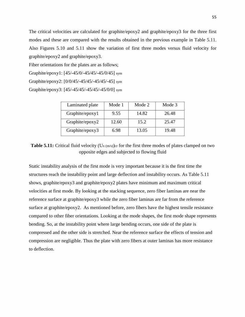
55

The critical velocities are calculated for graphite/epoxy2 and graphite/epoxy3 for the three first

modes and these are compared with the results obtained in the previous example in Table 5.11.

Also Figures 5.10 and 5.11 show the variation of first three modes versus fluid velocity for

graphite/epoxy2 and graphite/epoxy3.

Fiber orientations for the plates are as follows;

Graphite/epoxy1: [45/-45/0/-45/45/-45/0/45] sym

Graphite/epoxy2: [0/0/45/-45/45/-45/45/-45] sym

Graphite/epoxy3: [45/-45/45/-45/45/-45/0/0] sym

Laminated plate Mode 1 Mode 2 Mode 3

Graphite/epoxy1 9.55 14.82 26.48



Table 5.11: Critical fluid velocity (Ux (m/s))cr for the first three modes of plates clamped on two

opposite edges and subjected to flowing fluid

Static instability analysis of the first mode is very important because it is the first time the

structures reach the instability point and large deflection and instability occurs. As Table 5.11

shows, graphite/epoxy3 and graphite/epoxy2 plates have minimum and maximum critical

velocities at first mode. By looking at the stacking sequence, zero fiber laminas are near the

reference surface at graphite/epoxy3 while the zero fiber laminas are far from the reference

surface at graphite/epoxy2. As mentioned before, zero fibers have the highest tensile resistance

compared to other fiber orientations. Looking at the mode shapes, the first mode shape represents

bending. So, at the instability point where large bending occurs, one side of the plate is

compressed and the other side is stretched. Near the reference surface the effects of tension and

compression are negligible. Thus the plate with zero fibers at outer laminas has more resistance

to deflection.

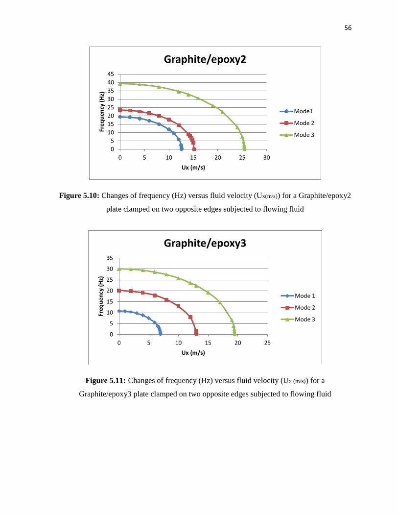
56

Figure 5.10: Changes of frequency (Hz) versus fluid velocity (Ux(m/s)) for a Graphite/epoxy2

plate clamped on two opposite edges subjected to flowing fluid

Figure 5.11: Changes of frequency (Hz) versus fluid velocity (Ux (m/s)) for a

Graphite/epoxy3 plate clamped on two opposite edges subjected to flowing fluid

0

5

10

15

20

25

30

35

40

45

0 5 10 15 20 25 30

Fre

qu

en

cy (

Hz)

Ux (m/s)

Graphite/epoxy2

Mode1

Mode 2

Mode 3

0

5

10

15

20

25

30

35

0 5 10 15 20 25

Fre

qu

en

cy (

Hz)

Ux (m/s)

Graphite/epoxy3

Mode 1

Mode 2

Mode 3

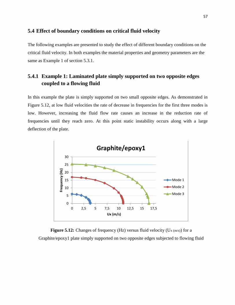
57

5.4 Effect of boundary conditions on critical fluid velocity

The following examples are presented to study the effect of different boundary conditions on the

critical fluid velocity. In both examples the material properties and geometry parameters are the

same as Example 1 of section 5.3.1.

5.4.1 Example 1: Laminated plate simply supported on two opposite edges

coupled to a flowing fluid

In this example the plate is simply supported on two small opposite edges. As demonstrated in

Figure 5.12, at low fluid velocities the rate of decrease in frequencies for the first three modes is

low. However, increasing the fluid flow rate causes an increase in the reduction rate of

frequencies until they reach zero. At this point static instability occurs along with a large

deflection of the plate.


Graphite/epoxy1 plate simply supported on two opposite edges subjected to flowing fluid

0

5

10

15

20

25

30

0 2,5 5 7,5 10 12,5 15 17,5

Fre

qu

en

cy (

Hz)

Ux (m/s)

Graphite/epoxy1

Mode 1

Mode 2

Mode 3

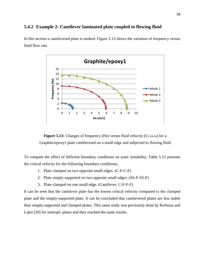
58

5.4.2 Example 2: Cantilever laminated plate coupled to flowing fluid

In this section a cantilevered plate is studied. Figure 5.13 shows the variation of frequency versus

fluid flow rate.


Graphite/epoxy1 plate cantilevered on a small edge and subjected to flowing fluid

To compare the effect of different boundary conditions on static instability, Table 5.12 presents

the critical velocity for the following boundary conditions;

1. Plate clamped on two opposite small edges. (C-F-C-F)

2. Plate simply supported on two opposite small edges. (SS-F-SS-F)

3. Plate clamped on one small edge. (Cantilever, C-F-F-F)

It can be seen that the cantilever plate has the lowest critical velocity compared to the clamped

plate and the simply-supported plate. It can be concluded that cantilevered plates are less stable

than simply-supported and clamped plates. This same study was previously done by Kerboua and

Lakis [20] for isotropic plates and they reached the same results.

0

2

4

6

8

10

12

14

16

0 1 2 3 4 5 6 7 8 9 10

Fre

qu

en

cy (

Hz)

Ux (m/s)

Graphite/epoxy1

Mode 1

Mode 2

Mode 3

59

Graphite/epoxy1 Critical velocity (Ux)cr

Boundary Condition /Mode Mode 1 Mode 2 Mode 3

C-F-C-F 9.55 14.82 26.48

SS-F-SS-F 3.92 10.99 16.51

C-F-F-F 1.46 5.94 8.78

Table 5.12: Critical fluid velocity (Ux (m/s))cr for the first three modes of Graphite/epoxy1 for

different boundary conditions

60

CHAPTER 6 CONCLUSION AND FUTURE WORK

The purpose of this study was to present an analysis of the dynamic behavior of laminated

composite and isotropic plates under different conditions including: totally submerged in fluid,

floating on fluid and in air (vacuo). Various boundary conditions were applied to a solid finite

element model and results were presented using figures and tables. Results of a study on the

effect of fiber orientation on the static instability of a structure were also presented.

The structural model in this work is described using classical laminated plate theory, Sander‘s

shell theory and the finite element method. The plate is composed of different layers with

different fiber orientations. Each lamina could be made of continuous, discontinuous and

discontinuous random fibers with different matrices, but in this investigation the same material

was used to build the laminas; the fibers were continuous (graphite) and matrices were made of

epoxy. The lay-up of laminas was symmetrical such that the resulting laminated composite plate

was balanced and symmetric. For our analysis, the plate was discretized into a number of

rectangular finite elements, each with 24 degrees of freedom (each of the 4 corner nodes had 6

degrees of freedom). Using exponential and bilinear polynomial functions, all out-of-plane and

in-plane displacements were modeled.

Potential fluid flow induced pressure on the structure. In turn, this pressure induced inertial,

Coriolis and centrifugal effects. To define this pressure as a function of transverse displacement,

acceleration and velocity, Laplace and Bernoulli equations and the impermeability condition

were used. Finally, the mass, stiffness and damping matrices were defined and relations for fluid-

solid-interactions were developed by exact mathematical integration for each element.

Modal analysis of several isotropic and laminated plates with different dimensions, stacking

sequences and boundary conditions were studied. Also, stability analysis was discussed in order

to find the critical velocity for structure. It was demonstrated that boundary conditions and fiber

orientation have a strong effect on the dynamic behavior of the structure; a cantilevered plate is

more likely to become unstable than plates with other boundary conditions under the same

loading arrangement. The plate under study was made of a kind of graphite/epoxy with laminas

with zero fiber orientations in the outer layers. These plates therefore had more resistance to

divergence compared to plates made with zero fiber lamina near the middle surface.

61

The natural vibration frequencies calculated in this study agree well with those obtained by

Lindholm, Crawley , Pal and an ANSYS model, especially for low modes.

As a future work, the present method could be further developed for other types of composite

materials such as non-symmetric laminated material or sandwich-laminated composites. Also the

boundary condition of the fluid could be changed so that the plate could be considered as

bounded by an elastic wall.

As another subject of future work, the stiffness matrix of plate could be developed using first-

order shear deformation theory (FSDT) or higher-order shear deformation theory (HSDT) and

compared with the results of the present study.

Also, the present method could be used for analyzing a situation involving forced vibration of the

plate while external forces are applied to the structure.

62

REFERENCES

[1] A.W. Leissa, "The free vibration of rectangular plates," Journal of Sound and Vibration,

vol. 31, pp. 257-293, 1973.

[2] J.N. Reddy, "Free vibration of antisymmetric, angle-ply laminated plates including

transverse shear deformation by the finite element method," Journal of Sound and

Vibration, vol. 66, pp. 565-576, 1979.

[3] W. Han and M. Petyt, "Linear vibration analysis of laminated rectangular plates using the

hierarchical finite element method—I. Free vibration analysis," Computers &

Structures, vol. 61, pp. 705-712, 1996.

[4] M.-H. Hsu, "Vibration analysis of isotropic and orthotropic plates with mixed boundary

conditions," Tamkang Journal of Science and Engineering, vol. 6, pp. 217-226, 2003.

[5] S. Xiang, Wang and Ke-Ming, Free vibration analysis of symmetric laminated composite

plates by trigonometric shear deformation theory and inverse multiquadric RBF vol. 47.

Kidlington, Royaume-uni: Elsevier, 2009.

[6] H. Lamb, "On the vibrations of an elastic plate in contact with water," Proceedings of the

Royal Society of London. Series A, Containing Papers of a Mathematical and Physical

Character, vol. 98, pp. 205-216, 1920.

[7] Y. Fu and W. G. Price, "Interactions between a partially or totally immersed vibrating

cantilever plate and the surrounding fluid," Journal of Sound and Vibration, vol. 118, pp.

495-513, 1987.

[8] A. A. Lakis and M. P. Païdoussis, "Free vibration of cylindrical shells partially filled with

liquid," Journal of Sound and Vibration, vol. 19, pp. 1-15, 1971.

[9] M. P. Paidoussis, Fluid-structure interactions between axial flows and slender structures,

1997.

[10] U. S. Lindholm, D. D. Kana, W.-H. Chu, and H. N. Abramson, "Elastic vibration

characteristics of cantilever plates in water," 1998.

[11] E. Charbonneau, "Analyse dynamique des plaques rectangulaires submergees dans un

fluide," M.Sc.A. MQ48843, Ecole Polytechnique, Montreal (Canada), Canada, 1999.

63

[12] M. H. Toorani and A. A. Lakis, "General equations of anisotropic plates and shells

including transverse shear deformations, rotary inertia and initial curvature effects,"

Journal of Sound and Vibration, vol. 237, pp. 561-615, 2000.

[13] M. H. Toorani and A. A. Lakis, "Dynamic analysis of anisotropic cylindrical shells

containing flowing fluid," Journal of Pressure Vessel Technology, vol. 123, pp. 454-460,

2001.

[14] Y. Kerboua, A. A. Lakis, M. Thomas, and L. Marcouiller, "Hybrid method for vibration

analysis of rectangular plates," Nuclear Engineering and Design, vol. 237, pp. 791-801,

2007.

[15] M. R. Haddara and S. Cao, "A study of the dynamic response of submerged rectangular

flat plates," Marine Structures, vol. 9, pp. 913-933, 1996.

[16] N. C. Pal, P. K. Sinha, and S. K. Bhattacharyya, "Finite element dynamic analysis of

submerged laminated composite plates," Journal of Reinforced Plastics and Composites,

vol. 20, pp. 547-563, May 1, 2001.

[17] N.-F.-N. Nguen-Fuk-Nin and G. A. Marchenko, "Flutter of an orthotropic cantilever plate

with stiffner ribs," International Applied Mechanics, vol. 6, pp. 562-564, 1970.

[18] P. Santini and P. Gasbarri, "Structural dynamics of a cantilever wing-like anisotropic

swept plate," Journal of Reinforced Plastics and Composites, vol. 19, pp. 1112-1146,

September 1, 2000.

[19] Y. Kerboua, A. A. Lakis, M. Thomas, L. Marcouiller, M. H. Toorani, and Asme, Critical

velocity of potential flow in interaction with a system of plates. New York: Amer Soc

Mechanical Engineers, 2009.

[20] Y. Kerboua, A. A. Lakis, M. Thomas, and L. Marcouiller, "Vibration analysis of

rectangular plates coupled with fluid," Applied Mathematical Modelling, vol. 32, pp.

2570-2586, 2008.

[21] Y. Kerboua, A. A. Lakis, M. Thomas, and L. Marcouiller, "Modelling of plates subjected

to flowing fluid under various boundary conditions," Engineering Applications of

Computational Fluid Mechanics, vol. 2, pp. 525-539, Dec 2008.

[22] P. K. Mallick, Fiber-reinforced composites : materials, manufacturing, and design. New

York: M. Dekker, 1988.

64

[23] J. N. Reddy, Mechanics of laminated composite plates and shells: theory and analysis:

CRC Press, 2004.

[24] R. M. Christensen, "The numbers of elastic properties and failure Pparameters for fiber

composites," Journal of Engineering Materials and Technology, vol. 120, pp. 110-113,

1998.

[25] H. Kraus, Thin elastic shells: an introduction to the theoretical foundations and the

analysis of their static and dynamic behavior: Wiley, 1967.

[26] J. M. Whitney and J. E. Ashton, Structural analysis of laminated anisotropic plates:

Technomic Pub. Co., 1987.

[27] M. H. Toorani and A. A. Lakis, "Shear deformation in dynamic analysis of anisotropic

laminated open cylindrical shells filled with or subjected to a flowing fluid," Computer

Methods in Applied Mechanics and Engineering, vol. 190, pp. 4929-4966, 2001.

[28] M. Esmailzadeh, A. A. Lakis, M. Thomas, and L. Marcouiller, "Three-dimensional

modeling of curved structures containing and/or submerged in fluid," Finite Elements in

Analysis and Design, vol. 44, pp. 334-345, 2008.

[29] E. F. Crawley, "The natural modes of graphite/epoxy cantilever plates and shells,"

Journal of Composite Materials, vol. 13, pp. 195-205, July 1, 1979.

[30] R. D. Blevins, Formulas for natural frequency and mode shape: Krieger Pub Co, 1979.

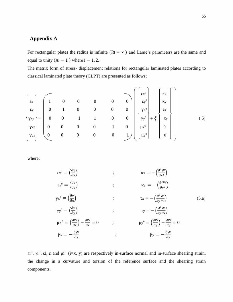
65

Appendix A

For rectangular plates the radius is infinite and Lame‘s parameters are the same and

equal to unity where .

The matrix form of stress- displacement relations for rectangular laminated plates according to

classical laminated plate theory (CLPT) are presented as follows;

1 0 0 0 0 0

0 0 0 0 0 x

0 0 + 𝜉 y ( 5)

0 0 0 0 0

0 0 0 0 0

where;

(

) ; (

)

(

) ; (

)

(

) ; (

) (5.a)

(

) ; (

)

(

)

; (

)

;

, , τ and (i=x, y) are respectively in-surface normal and in-surface shearing strain,

the change in a curvature and torsion of the reference surface and the shearing strain

components.

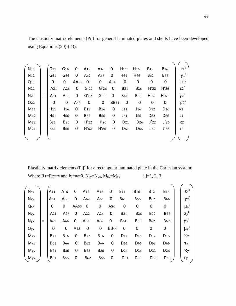
66

The elasticity matrix elements (Pij) for general laminated plates and shells have been developed

using Equations (20)-(23);

N11 G11 G16 0 A12 A16 0 H11 H16 B12 B16

N12 G61 G66 0 A62 A66 0 H61 H66 B62 B66

Q11 0 0 AA55 0 0 A54 0 0 0 0

N22 A21 A26 0 G’22 G’26 0 B21 B26 H’22 H’26

N21 = A61 A66 0 G’62 G’66 0 B61 B66 H’62 H’6 6

Q22 0 0 A45 0 0 BB44 0 0 0 0

M11 H11 H16 0 B12 B16 0 J11 J16 D12 D16

M12 H61 H66 0 B62 B66 0 J61 J66 D62 D66

M22 B21 B26 0 H’22 H’26 0 D21 D26 J’22 J’26

M21 B61 B66 0 H’62 H’66 0 D61 D66 J’62 J’66

Elasticity matrix elements (Pij) for a rectangular laminated plate in the Cartesian system;

Where R1=R2= and bi=ai=0, Nxy=Nyx, Mxy=Myx i,j=1, 2, 3

Nxx A11 A16 0 A12 A16 0 B11 B16 B12 B16

Nxy A61 A66 0 A62 A66 0 B61 B66 B62 B66

Qxx 0 0 AA55 0 0 A54 0 0 0 0

Nyy A21 A26 0 A22 A26 0 B21 B26 B22 B26

Nyx = A61 A66 0 A62 A66 0 B61 B66 B62 B6 6

Qyy 0 0 A45 0 0 BB44 0 0 0 0

Mxx B11 B16 0 B12 B16 0 D11 D16 D12 D16

Mxy B61 B66 0 B62 B66 0 D61 D66 D62 D66

Myy B21 B26 0 B22 B26 0 D21 D26 D22 D26

Myx B61 B66 0 B62 B66 0 D61 D66 D62 D66

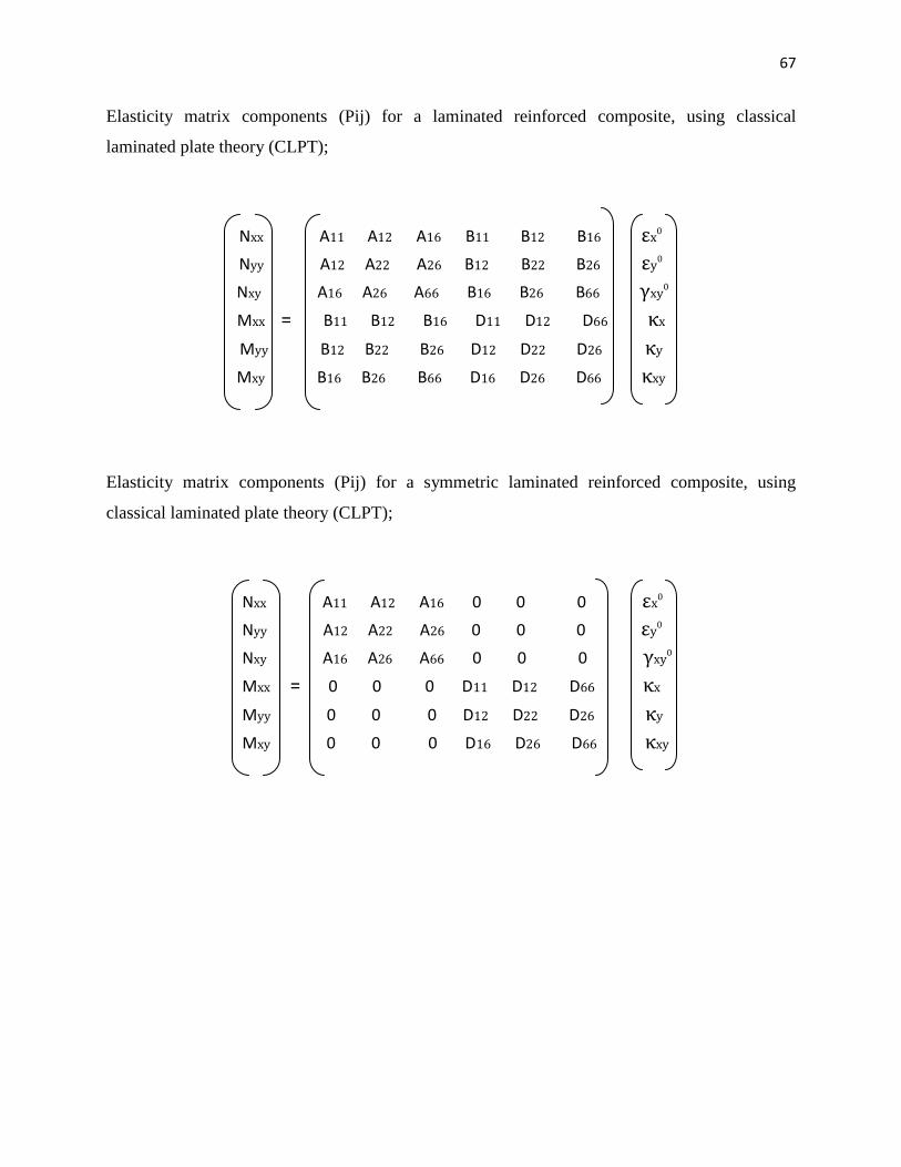
67

Elasticity matrix components (Pij) for a laminated reinforced composite, using classical

laminated plate theory (CLPT);

Nxx A11 A12 A16 B11 B12 B16

Nyy A12 A22 A26 B12 B22 B26

Nxy A16 A26 A66 B16 B26 B66

Mxx = B11 B12 B16 D11 D12 D66

Myy B12 B22 B26 D12 D22 D26

Mxy B16 B26 B66 D16 D26 D66

Elasticity matrix components (Pij) for a symmetric laminated reinforced composite, using

classical laminated plate theory (CLPT);

Nxx A11 A12 A16 0 0 0

Nyy A12 A22 A26 0 0 0

Nxy A16 A26 A66 0 0 0

Mxx = 0 0 0 D11 D12 D66

Myy 0 0 0 D12 D22 D26

Mxy 0 0 0 D16 D26 D66

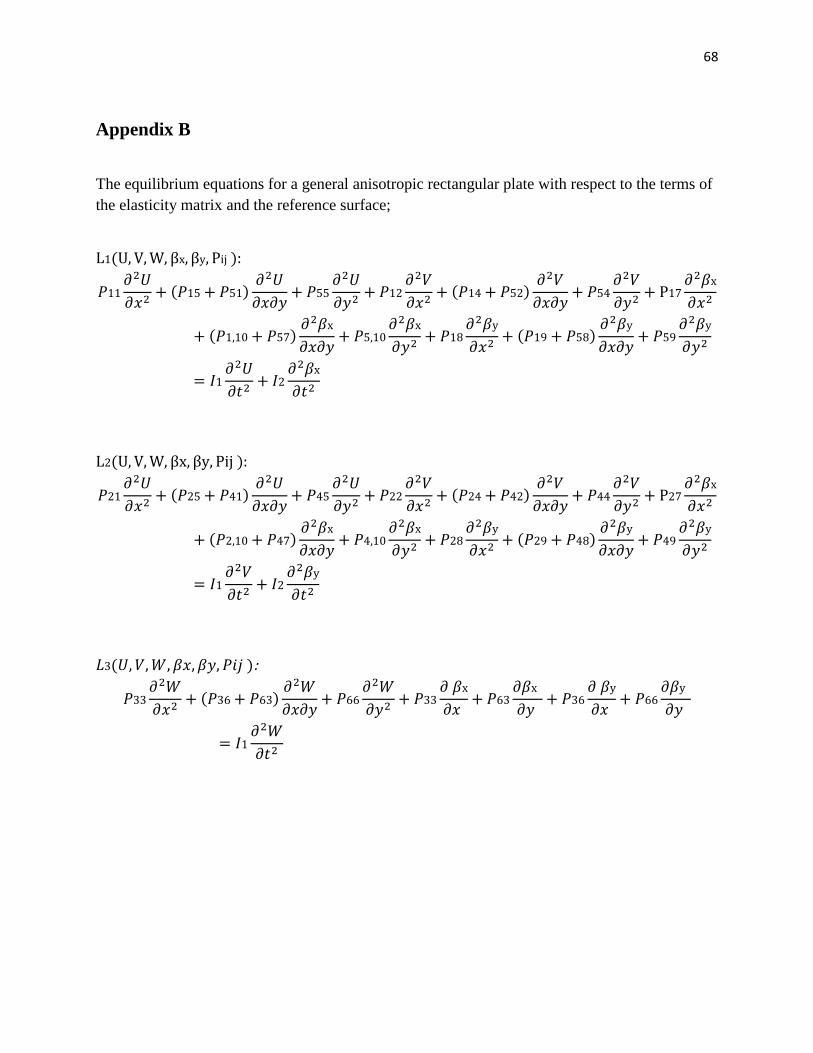
68

Appendix B

The equilibrium equations for a general anisotropic rectangular plate with respect to the terms of

the elasticity matrix and the reference surface;

:

𝛽

𝛽

𝛽

𝛽

𝛽

𝛽

𝛽

:

𝛽

𝛽

𝛽

𝛽

𝛽

𝛽

𝛽

𝛽 𝛽 :

𝛽

𝛽

𝛽

𝛽

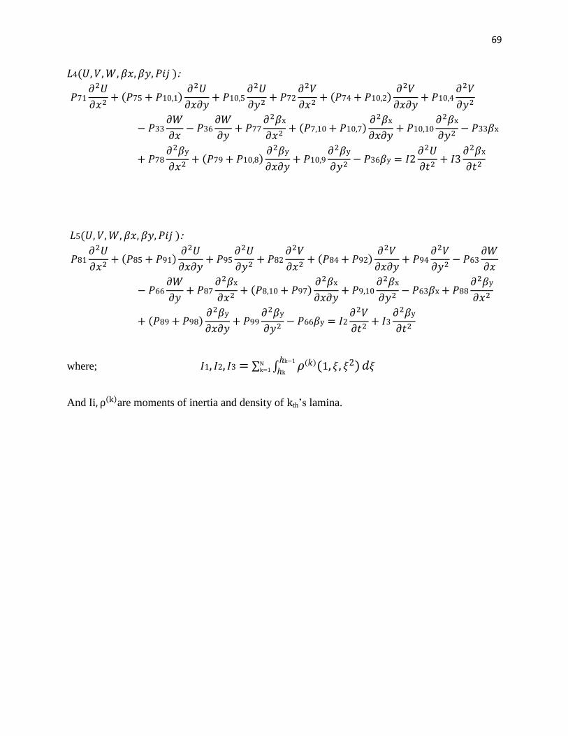
69

𝛽 𝛽 :

𝛽

𝛽

𝛽

𝛽

𝛽

𝛽

𝛽

𝛽

𝛽

𝛽 𝛽 :

𝛽

𝛽

𝛽

𝛽

𝛽

𝛽

𝛽

𝛽

𝛽

where; ∑ ∫ 𝜉 𝜉

𝜉

And are moments of inertia and density of th‘s lamina.

Documents

DYNAMIC ANALYSIS OF ISOTROPIC AND … ANALYSIS OF ISOTROPIC AND LAMINATED REINFORCED COMPOSITE PLATES ... 5.2 Modal analysis of plate totally ... Laminated plate simply supported …