Embed Size (px)
Citation preview
THÈSE NO 3285 (2005)
ÉCOLE POLYTECHNIQUE FÉDÉRALE DE LAUSANNE
PRÉSENTÉE À LA FACULTÉ INFORMATIQUE ET COMMUNICATIONS
Institut d'informatique fondamentale
SECTION DES SYSTÈMES DE COMMUNICATION
POUR L'OBTENTION DU GRADE DE DOCTEUR ÈS SCIENCES
PAR
ingénieur électricien diplômé EPFde nationalité suisse et originaire de Delémont (JU)
acceptée sur proposition du jury:
Lausanne, EPFL2005
Amre EL-HOIYDI
Prof. J.-D. Decotignie, directeur de thèseProf. J.-C. Grégoire, rapporteur
Dr A. Kaelin, rapporteurProf. A. Schiper, rapporteur
ENERGY EFFICIENT MEDIUM ACCESS CONTROL FOR WIRELESS SENSOR NETWORKS

iii
Acknowledgement
First of all, I would like to thank my advisor Prof. Jean-Dominique Decotignie, to have givenme the opportunity to pursue a PhD in his group. His far-seeing guidance directed my researchtowards an area that proved to be very interesting. I am grateful for his high availability andfor the support and trust he gave me.
Most of the work presented within this dissertation was made within the WiseNET projectat CSEM. I would like to thank all the participants of the WiseNET project. In particular, Iwould like to thank Erwan Le Roux for having spent many hours explaining me the workingsof the WiseNET system-on-chip and to have guided my work towards the preamble samplingtechnique, which proved to be a fruitful direction. Special thanks go also to Thierry Melly,Patrick Volet and Christian Enz.
Working in the Real-Time Software and Networking group at CSEM was a great pleasure.I am thankful to my colleagues in secteur 241 for there friendship and helpfulness. I wouldlike to thank particularly Jean Hernandez to have introduced me to the field of low powercommunication protocols.
I am grateful to Prof. Jean-Charles Gregoire, Dr. August Kaelin and Prof. Andre Schiper forhaving accepted to be part of my jury.
The work presented in this dissertation was supported (in part) by the National CompetenceCenter in Research on Mobile Information and Communication Systems (NCCR-MICS), a centersupported by the Swiss National Science Foundation under grant number 5005-67322.
This dissertation is dedicated to my son Felix, my wife Caroline and my parents Madeleineand Ahmed.
Amre El-HoiydiNeuchatel, July 2005

v
Abstract
A wireless sensor network designates a system composed of numerous sensor nodes distributedover an area in order to collect information. The sensor nodes communicate wirelessly with eachother in order to self-organize into a multi-hop network, collaborate in the sensing activity andforward the acquired information towards one or more users of the information. Applicationsof sensor networks are numerous, ranging from environmental monitoring, home and buildingautomation to industrial control.
Since sensor nodes are expected to be deployed in large numbers, they must be inexpensive.Communication between sensor nodes should be wireless in order to minimize the deploymentcost. The lifetime of sensor nodes must be long for minimal maintenance cost. The most im-portant consequence of the low cost and long lifetime requirements is the need for low powerconsumption. With today’s technology, wireless communication hardware consumes so muchpower that it is not acceptable to keep the wireless communication interface constantly in oper-ation. As a result, it is required to use a communication protocol with which sensor nodes areable to communicate keeping the communication interface turned-off most of the time.
The subject of this dissertation is the design of medium access control protocols permittingto reach a very low power consumption when communicating at a low average throughput inmulti-hop wireless sensor networks.
In a first part, the performance of a scheduled protocol (time division multiple access, TDMA)is compared to the one of a contention protocol (non-persistent carrier sensing multiple accesswith preamble sampling, NP-CSMA-PS). The preamble sampling technique is a scheme thatavoids constant listening to an idle medium. This thesis presents a low power contention protocolobtained through the combination of preamble sampling with non-persistent carrier sensingmultiple access. The analysis of the strengths and weaknesses of TDMA and NP-CSMA-PS ledus to propose a solution that exploits TDMA for the transport of frequent periodic data trafficand NP-CSMA-PS for the transport of sporadic signalling traffic required to setup the TDMAschedule.
The second part of this thesis describes the WiseMAC protocol. This protocol is a furtherenhancement of CSMA with preamble sampling that proved to provide both a low power con-sumption in low traffic conditions and a high energy efficiency in high traffic conditions. It isshown that this protocol can provide either a power consumption or a latency several times lowerthat what is provided by previously proposed protocols. The WiseMAC protocol was initiallydesigned for multi-hop wireless sensor networks. A comparison with power saving protocolsdesigned specifically for the downlink of infrastructure wireless networks shows that it is also ofinterest in such cases. An implementation of the WiseMAC protocol has permitted to validateexperimentally the proposed concepts and the presented analysis.

vii
Version abregee
Un reseau de capteurs sans fil est un systeme compose de nombreux capteurs distribues surune zone pour collecter de l’information. Les capteurs communiquent entre eux par ondes ra-dio pour auto-organiser la formation du reseau, pour collaborer dans les activites de mesure etpour acheminer l’information collectee vers un ou plusieurs utilisateurs de cette information.Les applications de reseaux de capteurs sans fil sont nombreuses. Elles comprennent notam-ment la surveillance de l’environnement naturel ou construit (agriculture, genie civil, etc) etl’automatisation dans les batiments (securite, controle de la ventilation, du chauffage, etc).
Pour pouvoir etre deployes en grand nombre, les capteurs doivent etre bon marche. La com-munication entre les capteurs doit se faire sans fil pour permettre un bas cout d’installation.La duree de vie d’un capteur doit etre longue pour minimiser les couts de maintenance. Laconsequence des ces besoins est que leur consommation en energie doit etre faible. Avec latechnologie actuelle, le materiel permettant une communication par ondes radio consomme unequantite d’energie telle qu’un fonctionnement permanent est inacceptable. Il est donc necessaired’utiliser un protocole de communication permettant aux capteurs de communiquer tout engardant leur interface radio eteinte la plupart du temps.
Cette dissertation a pour sujet la conception de protocoles de gestion d’acces permettant unetres faible consommation d’energie pour des communications a faible debit dans des reseaux decapteurs distribues.
Dans la premiere partie, les performances d’un protocole utilisant une organisation tem-porelle (multiplexage temporel, ou time division multiple access TDMA) sont comparees acelles d’un protocole utilisant une methode d’acces par competition (methode d’acces multi-ple avec ecoute de porteuse, sans persistance, et avec echantillonnage de preambule, ou non-persistent carrier sensing multiple access with preamble sampling NP-CSMA-PS). La techniquede l’echantillonnage de preambule permet d’eviter l’ecoute permanente d’un canal libre. Cettethese presente un protocole a basse consommation d’energie utilisant une methode d’acces parcompetition, obtenue en combinant la methode d’acces multiple avec ecoute de porteuse avec latechnique de l’echantillonnage de preambule. L’analyse des avantages et faiblesses des protocolesTDMA et NP-CSMA-PS a conduit a proposer une solution qui exploite a la fois le multiplexagetemporel pour le transport du trafic periodique et frequent des informations collectees, et lamethode d’acces par competition pour le transport du trafic sporadique utile a la mise en placedu multiplexage temporel.
La deuxieme partie de cette these decrit le protocole WiseMAC. Ce protocole est une versionamelioree de NP-CSMA-PS qui permet d’obtenir avec un seul protocole une tres basse consom-mation pour le transport de trafic sporadique et une haute efficacite energetique en cas de grandtrafic. Il est demontre que ce protocole permet d’obtenir une consommation energetique ou unelatence plusieurs fois inferieur a ce que permettent d’obtenir les protocoles proposes auparavant.

Ce protocole a ete concu initialement pour des reseaux a sauts multiples. Une comparaison avecles protocoles concus specifiquement pour le lien descendant de reseaux sans fil a infrastructurea demontre que WiseMAC est aussi interessant dans ces cas. Une implementation du protocoleWiseMAC a permit de valider experimentalement les concepts proposes et l’analyse presentee.

ix
Contents
List of Figures 13
List of Tables 17
1 Introduction 11.1 Topologies . . . . . . . . . . . . . . . . . . . . . . . . . . . . . . . . . . . . . . . . 11.2 Requirements . . . . . . . . . . . . . . . . . . . . . . . . . . . . . . . . . . . . . . 31.3 Low power design . . . . . . . . . . . . . . . . . . . . . . . . . . . . . . . . . . . . 41.4 Energy efficient communication . . . . . . . . . . . . . . . . . . . . . . . . . . . . 4
1.4.1 Physical layer . . . . . . . . . . . . . . . . . . . . . . . . . . . . . . . . . . 41.4.2 Data link layer . . . . . . . . . . . . . . . . . . . . . . . . . . . . . . . . . 51.4.3 Network layers . . . . . . . . . . . . . . . . . . . . . . . . . . . . . . . . . 51.4.4 Transport, session, and presentation layers . . . . . . . . . . . . . . . . . . 6
1.5 Problem statement . . . . . . . . . . . . . . . . . . . . . . . . . . . . . . . . . . . 61.6 Contributions . . . . . . . . . . . . . . . . . . . . . . . . . . . . . . . . . . . . . . 61.7 Thesis organization . . . . . . . . . . . . . . . . . . . . . . . . . . . . . . . . . . . 7
2 Energy Efficient Medium Access Control - State of the Art 92.1 Medium access control . . . . . . . . . . . . . . . . . . . . . . . . . . . . . . . . . 92.2 Sources of energy waste at MAC layer . . . . . . . . . . . . . . . . . . . . . . . . 102.3 Power saving schemes at MAC layer . . . . . . . . . . . . . . . . . . . . . . . . . 11
2.3.1 Wireless Local Area Networks (WLANs) . . . . . . . . . . . . . . . . . . . 112.3.1.1 IEEE 802.11 infrastructure mode . . . . . . . . . . . . . . . . . . 112.3.1.2 Hiperlan 2 . . . . . . . . . . . . . . . . . . . . . . . . . . . . . . 12
2.3.2 Mobile Ad-Hoc Networks (MANETs) . . . . . . . . . . . . . . . . . . . . 132.3.2.1 IEEE 802.11 ad-hoc mode . . . . . . . . . . . . . . . . . . . . . 132.3.2.2 Hiperlan 1 . . . . . . . . . . . . . . . . . . . . . . . . . . . . . . 14
2.3.3 Paging systems . . . . . . . . . . . . . . . . . . . . . . . . . . . . . . . . . 142.3.3.1 POCSAG . . . . . . . . . . . . . . . . . . . . . . . . . . . . . . . 142.3.3.2 FLEX and ERMES . . . . . . . . . . . . . . . . . . . . . . . . . 15
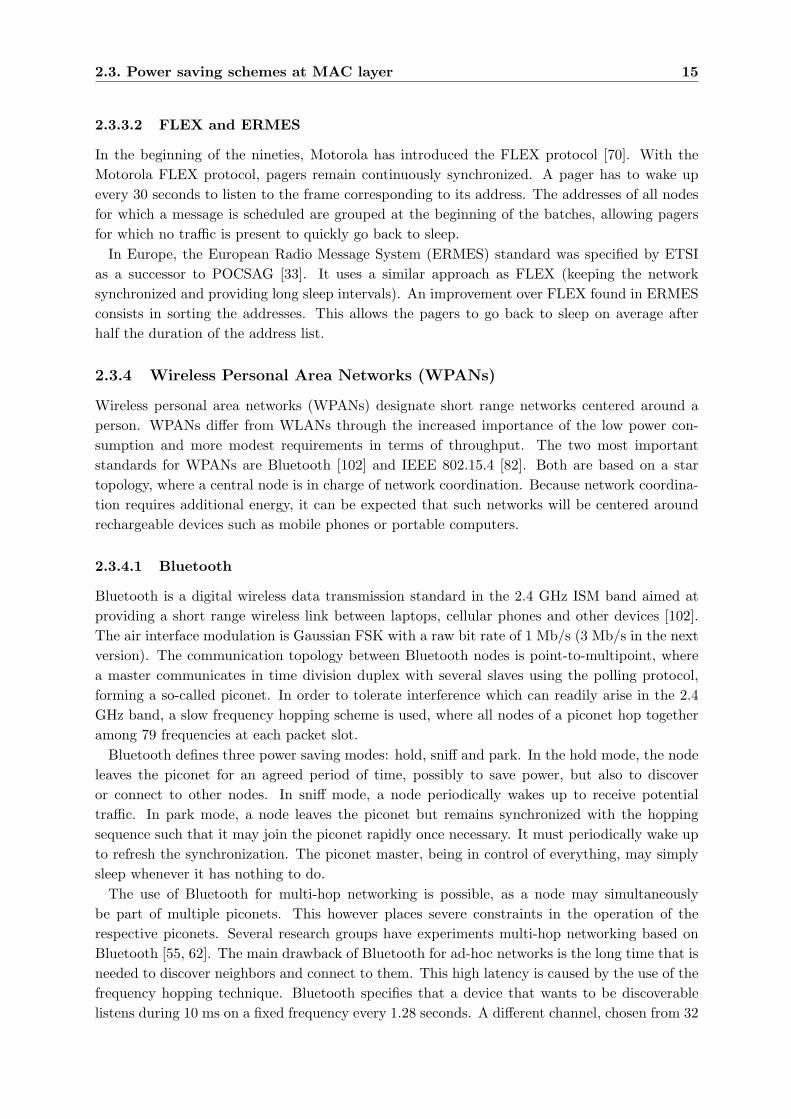
2.3.4 Wireless Personal Area Networks (WPANs) . . . . . . . . . . . . . . . . . 152.3.4.1 Bluetooth . . . . . . . . . . . . . . . . . . . . . . . . . . . . . . . 152.3.4.2 IEEE 802.15.4 . . . . . . . . . . . . . . . . . . . . . . . . . . . . 16
2.3.5 Wireless sensor networks . . . . . . . . . . . . . . . . . . . . . . . . . . . . 182.3.5.1 Scheduled MAC Protocols . . . . . . . . . . . . . . . . . . . . . 192.3.5.2 Unscheduled MAC Protocols . . . . . . . . . . . . . . . . . . . . 21
2.4 Summary . . . . . . . . . . . . . . . . . . . . . . . . . . . . . . . . . . . . . . . . 23
3 Battery and Transceiver Models 253.1 Introduction . . . . . . . . . . . . . . . . . . . . . . . . . . . . . . . . . . . . . . . 253.2 Battery model . . . . . . . . . . . . . . . . . . . . . . . . . . . . . . . . . . . . . 253.3 Radio transceiver model . . . . . . . . . . . . . . . . . . . . . . . . . . . . . . . . 26
3.3.1 Model parameters . . . . . . . . . . . . . . . . . . . . . . . . . . . . . . . 263.3.1.1 Power consumption and transition delays . . . . . . . . . . . . . 263.3.1.2 Other parameters . . . . . . . . . . . . . . . . . . . . . . . . . . 28
3.3.2 WiseNET SoC model . . . . . . . . . . . . . . . . . . . . . . . . . . . . . 293.4 Conclusion . . . . . . . . . . . . . . . . . . . . . . . . . . . . . . . . . . . . . . . 30
4 Spatial TDMA and Non-Persistent CSMA with Preamble Sampling 334.1 Introduction . . . . . . . . . . . . . . . . . . . . . . . . . . . . . . . . . . . . . . . 334.2 Spatial TDMA . . . . . . . . . . . . . . . . . . . . . . . . . . . . . . . . . . . . . 33
4.2.1 Scenario . . . . . . . . . . . . . . . . . . . . . . . . . . . . . . . . . . . . . 334.2.2 Required synchronization interval . . . . . . . . . . . . . . . . . . . . . . . 344.2.3 Power consumption . . . . . . . . . . . . . . . . . . . . . . . . . . . . . . . 35
4.3 Non-persistent CSMA with preamble sampling . . . . . . . . . . . . . . . . . . . 374.3.1 Preamble sampling . . . . . . . . . . . . . . . . . . . . . . . . . . . . . . . 374.3.2 Carrier sensing protocols . . . . . . . . . . . . . . . . . . . . . . . . . . . 384.3.3 Non-persistent CSMA with preamble sampling . . . . . . . . . . . . . . . 40
4.3.3.1 Throughput . . . . . . . . . . . . . . . . . . . . . . . . . . . . . 414.3.3.2 Delay . . . . . . . . . . . . . . . . . . . . . . . . . . . . . . . . . 424.3.3.3 Power consumption . . . . . . . . . . . . . . . . . . . . . . . . . 43
4.3.4 Regular and genie aided NP-CSMA . . . . . . . . . . . . . . . . . . . . . 444.3.5 Performance evaluation . . . . . . . . . . . . . . . . . . . . . . . . . . . . 454.3.6 Mitigating overhearing . . . . . . . . . . . . . . . . . . . . . . . . . . . . . 48
4.4 Comparing and combining S-TDMA and NP-CSMA-PS . . . . . . . . . . . . . . 49
5 WiseMAC for Multihop Wireless Sensor Networks 535.1 Introduction . . . . . . . . . . . . . . . . . . . . . . . . . . . . . . . . . . . . . . . 535.2 Protocol description . . . . . . . . . . . . . . . . . . . . . . . . . . . . . . . . . . 53
5.2.1 Overview . . . . . . . . . . . . . . . . . . . . . . . . . . . . . . . . . . . . 535.2.2 Minimized wake-up preamble . . . . . . . . . . . . . . . . . . . . . . . . . 545.2.3 Medium reservation . . . . . . . . . . . . . . . . . . . . . . . . . . . . . . 555.2.4 Random backoff . . . . . . . . . . . . . . . . . . . . . . . . . . . . . . . . 595.2.5 Overhearing mitigation . . . . . . . . . . . . . . . . . . . . . . . . . . . . 605.2.6 ”More” bit . . . . . . . . . . . . . . . . . . . . . . . . . . . . . . . . . . . 645.2.7 Inter-frame spaces . . . . . . . . . . . . . . . . . . . . . . . . . . . . . . . 645.2.8 Receive and carrier sense thresholds . . . . . . . . . . . . . . . . . . . . . 655.2.9 Sampling period . . . . . . . . . . . . . . . . . . . . . . . . . . . . . . . . 68
5.3 Performance analysis . . . . . . . . . . . . . . . . . . . . . . . . . . . . . . . . . . 695.3.1 Reference protocols . . . . . . . . . . . . . . . . . . . . . . . . . . . . . . . 70
5.3.1.1 Ideal protocol . . . . . . . . . . . . . . . . . . . . . . . . . . . . 705.3.1.2 S-MAC . . . . . . . . . . . . . . . . . . . . . . . . . . . . . . . . 71
5.3.1.3 T-MAC . . . . . . . . . . . . . . . . . . . . . . . . . . . . . . . . 715.3.1.4 CSMA/CA . . . . . . . . . . . . . . . . . . . . . . . . . . . . . . 72
5.3.2 Theoretical power consumption . . . . . . . . . . . . . . . . . . . . . . . . 725.3.2.1 Ideal protocol . . . . . . . . . . . . . . . . . . . . . . . . . . . . 735.3.2.2 S-MAC . . . . . . . . . . . . . . . . . . . . . . . . . . . . . . . . 735.3.2.3 WiseMAC . . . . . . . . . . . . . . . . . . . . . . . . . . . . . . 74
5.3.3 Simulation in a lattice network . . . . . . . . . . . . . . . . . . . . . . . . 765.3.3.1 Topology . . . . . . . . . . . . . . . . . . . . . . . . . . . . . . . 765.3.3.2 Traffic . . . . . . . . . . . . . . . . . . . . . . . . . . . . . . . . . 765.3.3.3 Receive, interference and carrier sense ranges . . . . . . . . . . . 775.3.3.4 Hop delay . . . . . . . . . . . . . . . . . . . . . . . . . . . . . . . 785.3.3.5 Power consumption . . . . . . . . . . . . . . . . . . . . . . . . . 795.3.3.6 Throughput . . . . . . . . . . . . . . . . . . . . . . . . . . . . . 815.3.3.7 Lifetime . . . . . . . . . . . . . . . . . . . . . . . . . . . . . . . . 815.3.3.8 Energy efficiency . . . . . . . . . . . . . . . . . . . . . . . . . . . 82
5.3.4 Simulation in a random network . . . . . . . . . . . . . . . . . . . . . . . 835.3.4.1 Topology and traffic . . . . . . . . . . . . . . . . . . . . . . . . . 835.3.4.2 Power consumption and delay . . . . . . . . . . . . . . . . . . . 84
5.4 Sensitivity analysis . . . . . . . . . . . . . . . . . . . . . . . . . . . . . . . . . . . 855.4.1 Impact of the sampling period . . . . . . . . . . . . . . . . . . . . . . . . 855.4.2 Impact of the different schemes used in WiseMAC . . . . . . . . . . . . . 865.4.3 Impact of external interferences . . . . . . . . . . . . . . . . . . . . . . . . 875.4.4 Importance of the transceiver parameters . . . . . . . . . . . . . . . . . . 885.4.5 Impact of the quartz frequency tolerance . . . . . . . . . . . . . . . . . . 885.4.6 Impact of the battery model . . . . . . . . . . . . . . . . . . . . . . . . . 89
5.5 Conclusion . . . . . . . . . . . . . . . . . . . . . . . . . . . . . . . . . . . . . . . 89
6 Downlink of an Infrastructure Wireless Sensor Network 916.1 Introduction . . . . . . . . . . . . . . . . . . . . . . . . . . . . . . . . . . . . . . . 91
6.1.1 Problem statement . . . . . . . . . . . . . . . . . . . . . . . . . . . . . . . 916.1.2 Traffic model . . . . . . . . . . . . . . . . . . . . . . . . . . . . . . . . . . 926.1.3 Chapter outline . . . . . . . . . . . . . . . . . . . . . . . . . . . . . . . . . 92
6.2 Low power downlink MAC protocols . . . . . . . . . . . . . . . . . . . . . . . . . 936.2.1 Ideal protocol . . . . . . . . . . . . . . . . . . . . . . . . . . . . . . . . . . 936.2.2 WiseMAC . . . . . . . . . . . . . . . . . . . . . . . . . . . . . . . . . . . . 946.2.3 Periodic Terminal Initiated Polling - PTIP . . . . . . . . . . . . . . . . . 946.2.4 IEEE 802.11/802.15.4 Power Save Mode - PSM . . . . . . . . . . . . . . . 956.2.5 Adaptability of the wake-up period . . . . . . . . . . . . . . . . . . . . . . 97
6.3 Power consumption . . . . . . . . . . . . . . . . . . . . . . . . . . . . . . . . . . . 976.3.1 Power consumption of the ideal protocol . . . . . . . . . . . . . . . . . . . 976.3.2 Power consumption of WiseMAC . . . . . . . . . . . . . . . . . . . . . . . 986.3.3 Power consumption of PTIP . . . . . . . . . . . . . . . . . . . . . . . . . 986.3.4 Power consumption of PSM . . . . . . . . . . . . . . . . . . . . . . . . . . 100
6.4 Transmission delay . . . . . . . . . . . . . . . . . . . . . . . . . . . . . . . . . . . 1006.4.1 Delay with the ideal protocol . . . . . . . . . . . . . . . . . . . . . . . . . 1006.4.2 Delay with WiseMAC . . . . . . . . . . . . . . . . . . . . . . . . . . . . . 101
6.4.3 Delay with PTIP . . . . . . . . . . . . . . . . . . . . . . . . . . . . . . . . 1026.4.4 Delay with PSM . . . . . . . . . . . . . . . . . . . . . . . . . . . . . . . . 103
6.5 Performance comparison . . . . . . . . . . . . . . . . . . . . . . . . . . . . . . . . 1036.6 Sensitivity analysis . . . . . . . . . . . . . . . . . . . . . . . . . . . . . . . . . . . 106
6.6.1 Sensitivity to traffic . . . . . . . . . . . . . . . . . . . . . . . . . . . . . . 1066.6.2 Scalability . . . . . . . . . . . . . . . . . . . . . . . . . . . . . . . . . . . . 1066.6.3 Impact of the data frame repetition in the WiseMAC preamble . . . . . . 1086.6.4 Impact of the packet size . . . . . . . . . . . . . . . . . . . . . . . . . . . 1106.6.5 Impact of the quartz frequency tolerance . . . . . . . . . . . . . . . . . . 1116.6.6 Impact of the TX/RX power consumption ratio . . . . . . . . . . . . . . . 1116.6.7 Impact of the bit rate . . . . . . . . . . . . . . . . . . . . . . . . . . . . . 112
6.7 Conclusion . . . . . . . . . . . . . . . . . . . . . . . . . . . . . . . . . . . . . . . 114
7 Experimentation 1177.1 Introduction . . . . . . . . . . . . . . . . . . . . . . . . . . . . . . . . . . . . . . . 1177.2 Hardware platform . . . . . . . . . . . . . . . . . . . . . . . . . . . . . . . . . . . 117
7.2.1 Microcontroller . . . . . . . . . . . . . . . . . . . . . . . . . . . . . . . . . 1177.2.2 Radio transceiver . . . . . . . . . . . . . . . . . . . . . . . . . . . . . . . . 1187.2.3 Development and demonstration boards . . . . . . . . . . . . . . . . . . . 119
7.3 Software architecture . . . . . . . . . . . . . . . . . . . . . . . . . . . . . . . . . . 1197.4 Measurements . . . . . . . . . . . . . . . . . . . . . . . . . . . . . . . . . . . . . . 120
7.4.1 Time-keeping base accuracy . . . . . . . . . . . . . . . . . . . . . . . . . . 1207.4.2 Static current consumption . . . . . . . . . . . . . . . . . . . . . . . . . . 1207.4.3 Dynamic current consumption . . . . . . . . . . . . . . . . . . . . . . . . 1217.4.4 Energy consumption of sampling . . . . . . . . . . . . . . . . . . . . . . . 1237.4.5 Minimization of the wake-up preamble length . . . . . . . . . . . . . . . . 1237.4.6 Multi-hop transmission . . . . . . . . . . . . . . . . . . . . . . . . . . . . 1257.4.7 Average power consumption and transmission delay . . . . . . . . . . . . 126
7.5 Conclusion . . . . . . . . . . . . . . . . . . . . . . . . . . . . . . . . . . . . . . . 128
8 Conclusion 129
A Interference Between Bluetooth Piconets 131A.1 Introduction . . . . . . . . . . . . . . . . . . . . . . . . . . . . . . . . . . . . . . . 131A.2 Model . . . . . . . . . . . . . . . . . . . . . . . . . . . . . . . . . . . . . . . . . . 131A.3 Packet Error Rate . . . . . . . . . . . . . . . . . . . . . . . . . . . . . . . . . . . 132A.4 Aggregated Throughput . . . . . . . . . . . . . . . . . . . . . . . . . . . . . . . . 136A.5 Simulation Model in OPNET . . . . . . . . . . . . . . . . . . . . . . . . . . . . . 136A.6 Simulations Results . . . . . . . . . . . . . . . . . . . . . . . . . . . . . . . . . . . 139A.7 Conclusion . . . . . . . . . . . . . . . . . . . . . . . . . . . . . . . . . . . . . . . 141
B Simulation Model 143B.1 Simulation plateform . . . . . . . . . . . . . . . . . . . . . . . . . . . . . . . . . . 143B.2 Interference and radio layer simulation model . . . . . . . . . . . . . . . . . . . . 143
Bibliography 147
xiii
List of Figures
1.1 Sensor network topologies. . . . . . . . . . . . . . . . . . . . . . . . . . . . . . . . 2
2.1 IEEE 802.11 infrastructure network, power saving mode for downlink communi-cation. . . . . . . . . . . . . . . . . . . . . . . . . . . . . . . . . . . . . . . . . . . 12
2.2 Power saving in an IEEE 802.11 ad-hoc network. . . . . . . . . . . . . . . . . . . 132.3 POCSAG paging system frame format. . . . . . . . . . . . . . . . . . . . . . . . . 142.4 IEEE 802.15.4 beacon-enabled superframe structure. . . . . . . . . . . . . . . . . 162.5 Downlink data transfer in a beacon-enabled IEEE 802.15.4 network. . . . . . . . 162.6 Uplink data transfer in a beacon-enabled IEEE 802.15.4 network. . . . . . . . . . 172.7 A classification of MAC protocols for wireless sensor networks. . . . . . . . . . . 192.8 S-MAC. . . . . . . . . . . . . . . . . . . . . . . . . . . . . . . . . . . . . . . . . . 212.9 Piconet. . . . . . . . . . . . . . . . . . . . . . . . . . . . . . . . . . . . . . . . . . 222.10 Operation of the paging channel in STEM. . . . . . . . . . . . . . . . . . . . . . 23
3.1 Typical discharge curve for alkaline/manganese batteries (left) and for lithium/manganesebatteries (right). . . . . . . . . . . . . . . . . . . . . . . . . . . . . . . . . . . . . 26
3.2 Lifetime of a sensor node using a single 2.6 Ah alkaline battery as a function ofthe average consumed power. . . . . . . . . . . . . . . . . . . . . . . . . . . . . . 27
3.3 Transceiver states, power consumption and transition delays. . . . . . . . . . . . 273.4 Current consumption of the WiseNET SoC during setup phase into receive state. 30
4.1 Spatial TDMA. . . . . . . . . . . . . . . . . . . . . . . . . . . . . . . . . . . . . . 344.2 TDMA communication with earlier listening for clock drift compensation. . . . . 344.3 Required synchronization period due to source and destination clock drifts. T is
the target transmission time. TS1 and TS2 are the early and late limits for thestart of the transmission by the source. TD is the target time for listening at thedestination. TD1 and TD2 are the early and late limits for the effective start ofthe listening phase by the destination. . . . . . . . . . . . . . . . . . . . . . . . . 36
4.4 Power consumption and lifetime with the TDMA protocol, when forwarding 60bytes packet every L seconds using the WiseNET transceiver. . . . . . . . . . . . 37
4.5 Preamble Sampling. . . . . . . . . . . . . . . . . . . . . . . . . . . . . . . . . . . 374.6 Residual vulnerability period with CSMA. . . . . . . . . . . . . . . . . . . . . . . 394.7 Non-persistent CSMA with preamble sampling. . . . . . . . . . . . . . . . . . . . 414.8 System model for NP-CSMA analysis. . . . . . . . . . . . . . . . . . . . . . . . . 414.9 Initial waiting delay and waiting delay for retransmissions with NP-CSMA. . . . 43
4.10 Performance of non-persistent CSMA with preamble sampling, as compared toclassical NP-CSMA and genie aided NP-CSMA. . . . . . . . . . . . . . . . . . . . 46
4.11 Power consumption as a function of the interval between successful transmissions. 474.12 Approximation without considering collisions. . . . . . . . . . . . . . . . . . . . . 474.13 Percentage of the time spent by the transceiver its different states using NP-
CSMA-PS, as a function of the packet inter-arrival. . . . . . . . . . . . . . . . . . 484.14 Comparison between the power consumption of TDMA and NP-CSMA-PS. . . . 504.15 Lifetime using Spatial TDMA and NP-CSMA-PS as a function of the data and
signalling traffic. . . . . . . . . . . . . . . . . . . . . . . . . . . . . . . . . . . . . 51
5.1 Minimizing the wake-up preamble length. . . . . . . . . . . . . . . . . . . . . . . 545.2 Clock drift compensation. . . . . . . . . . . . . . . . . . . . . . . . . . . . . . . . 555.3 Packet format. . . . . . . . . . . . . . . . . . . . . . . . . . . . . . . . . . . . . . 555.4 Adaptivity of the per-packet overhead to the traffic. . . . . . . . . . . . . . . . . 565.5 Systematic collision between two nodes transmitting to the same destination at
the same sampling time (A) and medium reservation (B). . . . . . . . . . . . . . 565.6 Probability for a node to capture the medium, defer its transmission or enter
in collision, for different number of contenders and as a function of the mediumreservation window size. The markers show simulation results. . . . . . . . . . . 58
5.7 Computation of the energy consumption of a collision resolution. . . . . . . . . . 585.8 Energy consumption per node (upper plot) and number of required contentions
per node (lower plot) with a contention resolution between C nodes. . . . . . . . 595.9 Probabilistic overhearing avoidance. . . . . . . . . . . . . . . . . . . . . . . . . . 615.10 Repetition of data message within wake-up preamble. . . . . . . . . . . . . . . . 615.11 Duration of the overhearing period with WiseMAC, when TP < TD (A), TD ≤
TP < TW − TD (B) and TW − TD ≤ TP ≤ TW (C). . . . . . . . . . . . . . . . . . 625.12 Average power wasted by a node overhearing transmissions, as a function of the
interval between transmissions (TW = 50, 200, 500 ms, TD = 19.2 ms). . . . . . . 635.13 Transmission of packet bursts using the ”more” bit. . . . . . . . . . . . . . . . . 655.14 Extended carrier sensing range for hidden node effect mitigation. . . . . . . . . . 675.15 Receiving, interfering and sensing range (upper plot) and receive threshold as a
function of the decay index (lower plot). . . . . . . . . . . . . . . . . . . . . . . . 685.16 Effect of a wrong estimation of the decay index. The estimated decay index used
to compute the receive threshold is equal to 3.5 in both cases. The effective decayindex is equal to 3 on the left plot, and to 4 and the right plot. . . . . . . . . . . 69
5.17 Lifetime when sampling the medium with period TW (no traffic). . . . . . . . . . 695.18 Ideal Protocol. . . . . . . . . . . . . . . . . . . . . . . . . . . . . . . . . . . . . . 705.19 Required duration for the listen interval in S-MAC. . . . . . . . . . . . . . . . . . 725.20 T-MAC inactivity timeout. . . . . . . . . . . . . . . . . . . . . . . . . . . . . . . 735.21 Overhearing duration TO as a function of the preamble duration TP (TW =
100 ms, TD = 19.2 ms). . . . . . . . . . . . . . . . . . . . . . . . . . . . . . . . . 765.22 Lattice network topology. . . . . . . . . . . . . . . . . . . . . . . . . . . . . . . . 775.23 Hop delay as a function of the injected traffic (packets have a length of 60 bytes,
TW = 100 ms). . . . . . . . . . . . . . . . . . . . . . . . . . . . . . . . . . . . . . 795.24 Average power consumption as a function of the injected traffic (packets have a
length of 60 bytes, TW = 100 ms). . . . . . . . . . . . . . . . . . . . . . . . . . . 80
5.25 Average throughput as a function of the injected traffic (packets payloads have alength of 46 bytes, TW = 100 ms). . . . . . . . . . . . . . . . . . . . . . . . . . . 81
5.26 Lifetime as a function of the traffic when using a single AA alkaline battery leaking10% of its initial capacity every year. . . . . . . . . . . . . . . . . . . . . . . . . . 82
5.27 Energy efficiency. . . . . . . . . . . . . . . . . . . . . . . . . . . . . . . . . . . . . 835.28 Random network topology. . . . . . . . . . . . . . . . . . . . . . . . . . . . . . . 845.29 Average power consumption. . . . . . . . . . . . . . . . . . . . . . . . . . . . . . 855.30 Average end-to-end delay. . . . . . . . . . . . . . . . . . . . . . . . . . . . . . . . 855.31 Power consumption (left) and delay (right) with WiseMAC as a function of traffic
intensity with different sampling periods TW =50, 100, 200, 500 ms. . . . . . . . 865.32 Throughput (top, left), delay (top, right), power consumption (bottom, left) and
lifetime (bottom, right) with WiseMAC as a function of traffic intensity withoutone of the following schemes: Wake-up preamble minimization, extended carriersensing, more bit, mandatory inter-frame space before transmission. . . . . . . . 87
5.33 Power consumption (left) and lifetime (right) with different values for the quartztolerance: θ = 30, 50 and 100 ppm. . . . . . . . . . . . . . . . . . . . . . . . . . . 88
5.34 Lifetime as a function of the traffic intensity when using a single AA alkalinebattery leaking 3% of its initial capacity every year. . . . . . . . . . . . . . . . . 89
6.1 Infrastructure wireless sensor network. . . . . . . . . . . . . . . . . . . . . . . . . 926.2 Downlink traffic model. . . . . . . . . . . . . . . . . . . . . . . . . . . . . . . . . 936.3 Ideal protocol. . . . . . . . . . . . . . . . . . . . . . . . . . . . . . . . . . . . . . 946.4 WiseMAC for the downlink of an infrastructure network. . . . . . . . . . . . . . . 956.5 WiseMAC: Transmission of several packets using the more bit. . . . . . . . . . . 956.6 Periodic Terminal Initiated Polling (PTIP). . . . . . . . . . . . . . . . . . . . . . 966.7 Optimized Power Save Mode (PSM). . . . . . . . . . . . . . . . . . . . . . . . . . 976.8 Power consumption and delay of WiseMAC, PTIP and PSM as a function of the
wake-up period TW (L = 1000 s). . . . . . . . . . . . . . . . . . . . . . . . . . . . 1046.9 Power-delay characteristics of WiseMAC, PTIP and PSM (L = 1000 s). . . . . . 1056.10 Power consumption as a function of the inter-arrival L (TW = 1 s). . . . . . . . . 1076.11 Power consumption as a function of the number of sensor nodes N , for different
values of L (TW = 1 s). . . . . . . . . . . . . . . . . . . . . . . . . . . . . . . . . 1086.12 Power consumption as a function of the inter-arrival L when data frames are not
repeated in the wake-up preamble (TW = 1 s). . . . . . . . . . . . . . . . . . . . . 1096.13 Power consumption as a function of the number of sensor nodes N , for different
values of L (TW = 1 s). . . . . . . . . . . . . . . . . . . . . . . . . . . . . . . . . 1106.14 Power delay characteristics of WiseMAC, PTIP and PSM for L = 1000 s and
θ = 10, 30, 100 ppm. A larger power consumption corresponds to a larger θ. . . . 1116.15 Power consumption of WiseMAC, PTIP and PSM for L = 1000 s as a function
of the P T /PR ratio. The chosen wake-up period is TW = 5 s to remain in thevalidity domain of PTIP. . . . . . . . . . . . . . . . . . . . . . . . . . . . . . . . . 112
6.16 Power-delay characteristics of WiseMAC, PTIP and PSM when using a 11 MbpsLucent Orinoco IEEE 802.11 transceiver (left) and a 250 kbps Chipcon CC2420802.15.4 transceiver (right). The inter-arrival time is L = 1000 s. . . . . . . . . . 113
6.17 Power consumption of a Lucent Orinoco IEEE 802.11 PC Card during the recep-tion of a beacon. . . . . . . . . . . . . . . . . . . . . . . . . . . . . . . . . . . . . 114
7.1 Simplified hardware architecture of a XE88LC06A microcontroller. . . . . . . . . 1187.2 EV108 Development board with XM1203 radio module. . . . . . . . . . . . . . . 1197.3 WiseNode: A miniaturized low power wireless sensor node based on the XE1203
radio and the XE88LC06A micro-controller. . . . . . . . . . . . . . . . . . . . . . 1197.4 Single (left) and dual (right) controller solution. . . . . . . . . . . . . . . . . . . . 1207.5 Code size in words of the different software components. . . . . . . . . . . . . . . 1207.6 Current consumption of a XE1203F radio driven by a XE88LC06A micro-controller
when traveling clock-wise (left, doze-receive-transmit-doze) and anti-clockwise(right, doze-transmit-receive-doze) in the transceiver state machine. . . . . . . . . 122
7.7 Current consumed by the XE1203 radio transceiver (thick line) and total con-sumed current (XE1203 and XE88LC06A) when sampling the medium. . . . . . 123
7.8 Transmission with wake-up preamble of the length of the sampling period (left)and transmission with a wake-up preamble of minimized size (right) (TW = 250 ms).124
7.9 Detailed view of a transmission with a wake-up preamble of minimized size. . . . 1257.10 Multi-hop transmission of a packet (TW = 250 ms). . . . . . . . . . . . . . . . . . 1267.11 Topology used for average power consumption and average delay measurements. 1277.12 Average power consumption, computed from the measured time spent with the
radio in receive and transmit states (TW = 250 ms). . . . . . . . . . . . . . . . . 1277.13 Average hop transmission delay measured in a circular network composed of 5
nodes (TW = 250 ms). . . . . . . . . . . . . . . . . . . . . . . . . . . . . . . . . . 127
A.1 Interference between piconets. . . . . . . . . . . . . . . . . . . . . . . . . . . . . . 132A.2 Single or double exposition to interference. . . . . . . . . . . . . . . . . . . . . . . 133A.3 Packet error rate suffered by one piconet because of the interference from n − 1
adversary piconets. . . . . . . . . . . . . . . . . . . . . . . . . . . . . . . . . . . . 135A.4 Packet error rate suffered by one piconet because of the interference from n − 1
unsynchronized adversary piconets (r = 366/625) for different values of the trafficG. . . . . . . . . . . . . . . . . . . . . . . . . . . . . . . . . . . . . . . . . . . . . 135
A.5 Aggregated throughput. . . . . . . . . . . . . . . . . . . . . . . . . . . . . . . . . 136A.6 Network topology with 9 interfering piconets. . . . . . . . . . . . . . . . . . . . . 137A.7 Network topology with 49 interfering piconets. . . . . . . . . . . . . . . . . . . . 138A.8 Source process model. . . . . . . . . . . . . . . . . . . . . . . . . . . . . . . . . . 138A.9 Sink process model. . . . . . . . . . . . . . . . . . . . . . . . . . . . . . . . . . . 139A.10 Jammer process model. . . . . . . . . . . . . . . . . . . . . . . . . . . . . . . . . 139A.11 Simulation results for jammers transmitting with a power of 2 W. . . . . . . . . 140A.12 Simulation results for jammers transmitting with a power of 20 mW. . . . . . . . 140
B.1 Transceiver simulation model . . . . . . . . . . . . . . . . . . . . . . . . . . . . . 144B.2 Accumulated noise. . . . . . . . . . . . . . . . . . . . . . . . . . . . . . . . . . . . 145B.3 Accumulated noise simulation model. . . . . . . . . . . . . . . . . . . . . . . . . . 145
xvii
List of Tables
3.1 Parameters used for the WiseNET SoC model. . . . . . . . . . . . . . . . . . . . 30
5.1 Comparison for L = 100 s . . . . . . . . . . . . . . . . . . . . . . . . . . . . . . . 80
6.1 Transceiver Parameters . . . . . . . . . . . . . . . . . . . . . . . . . . . . . . . . 113
7.1 Effective 32kHz quartz oscillation frequency . . . . . . . . . . . . . . . . . . . . . 1217.2 Measured static current consumption of XE88LC06A and XE1203 (3 V). . . . . 1217.3 XE88LC06A and XE1203F two-chips solution. . . . . . . . . . . . . . . . . . . . 122
A.1 n maximizing the aggregated throughput. . . . . . . . . . . . . . . . . . . . . . . 136

Chapter 1
Introduction
A Wireless Sensor Network (WSN) designates a system composed of numerous sensor nodesdistributed over an area in order to collect information [88, 89, 3]. The sensor nodes communicatewirelessly with each other to self-organize into a multi-hop network, collaborate in the sensingactivity and forward the acquired information towards one or more users of the information.Applications of sensor networks are numerous, ranging from environmental monitoring, homeand building automation to industrial control [52].
The main requirements of sensor nodes is a low power consumption, allowing a lifetime ofseveral years on a single small sized low-cost battery. As will be seen in the following chapters,a low power consumption is made possible, from the communication point of view, through alimitation of the traffic at application layer and through the acceptation of some latency whencommunicating. We will consider that the generated traffic will be low in average, not excludinghowever short high traffic periods.
The realization of wireless sensor networks presents many challenges. One of them is thedesign of communication protocols fulfilling their specific needs. A communication protocolstack is usually designed following the OSI 7 layer reference model [38]. The first four layers(1-4) are responsible of the information transport (single hop bit transfer at the physical layer,single hop packet transfer at the data link layer, multi-hop packet transfer at network layer,and reliable end-to-end packet transfer at transport layer). The remaining three layers (5-7) areresponsible of the management of the communication. This dissertation deals with the designof energy efficient medium access control (MAC) for wireless sensor networks. A MAC protocolis located in the second layer (data link) of the OSI model.
This chapter introduces the different network topologies that can be taken by a sensor networkand the requirements of sensor network applications. The main requirement, which is low powerconsumption, is discussed in more detail in the context of communication protocols. The fieldof this research is introduced, as well as its contributions.
1.1 Topologies
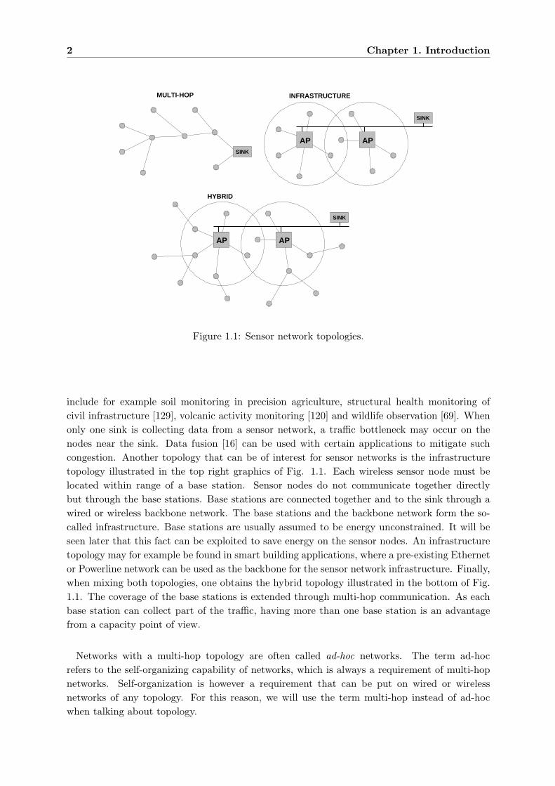
The classical topology that researchers consider when dealing with wireless sensor networks isthe multi-hop topology illustrated in the top left graphics of Fig. 1.1. With this topology, thesensor network does not rely on any fixed infrastructure. The acquired information is forwardedtowards a collection point called a sink. In this figure, a single collection point is depicted. Usingmultiple sinks in a sensor network is also possible. Applications of such a multi-hop topology
2 Chapter 1. Introduction
INFRASTRUCTUREMULTI-HOP
AP AP
AP AP
HYBRID
SINK
SINK
SINK
Figure 1.1: Sensor network topologies.
include for example soil monitoring in precision agriculture, structural health monitoring ofcivil infrastructure [129], volcanic activity monitoring [120] and wildlife observation [69]. Whenonly one sink is collecting data from a sensor network, a traffic bottleneck may occur on thenodes near the sink. Data fusion [16] can be used with certain applications to mitigate suchcongestion. Another topology that can be of interest for sensor networks is the infrastructuretopology illustrated in the top right graphics of Fig. 1.1. Each wireless sensor node must belocated within range of a base station. Sensor nodes do not communicate together directlybut through the base stations. Base stations are connected together and to the sink through awired or wireless backbone network. The base stations and the backbone network form the so-called infrastructure. Base stations are usually assumed to be energy unconstrained. It will beseen later that this fact can be exploited to save energy on the sensor nodes. An infrastructuretopology may for example be found in smart building applications, where a pre-existing Ethernetor Powerline network can be used as the backbone for the sensor network infrastructure. Finally,when mixing both topologies, one obtains the hybrid topology illustrated in the bottom of Fig.1.1. The coverage of the base stations is extended through multi-hop communication. As eachbase station can collect part of the traffic, having more than one base station is an advantagefrom a capacity point of view.
Networks with a multi-hop topology are often called ad-hoc networks. The term ad-hocrefers to the self-organizing capability of networks, which is always a requirement of multi-hopnetworks. Self-organization is however a requirement that can be put on wired or wirelessnetworks of any topology. For this reason, we will use the term multi-hop instead of ad-hocwhen talking about topology.
1.2. Requirements 3
1.2 Requirements
The requirements put on a sensor network vary from application to application. It is generallyadmitted [88, 89, 17, 3, 52] that the following requirements are set by most applications of sensornetworks:
• Low cost. For some applications, a cost per node of 100 Euros is acceptable. For mostapplications, the cost should be reduced as much as possible into the direction of 1 Europer node or less.
• Long lifetime. In many applications, it will not be possible or too expensive to replaceor recharge the battery of sensor nodes. The required lifetime depends on the application.A lifetime of a few month can already be useful for certain measurement campaigns. Inmost applications, a lifetime of a few years or more is desired.
• Large networks. Many sensor networks can be expected to be composed only of tens ofnodes. However, some applications may require sensor networks composed of hundreds orthousands of nodes. Sensor networks may also be large in the sense that the covered areais large.
The application requirements listed above lead to the following system requirements:
• Low power consumption: If sensor nodes are battery powered, the low cost require-ment imply to use mass produced batteries of modest capacity. As a long lifetime mustbe reached with batteries of modest capacity, it is crucial to minimize the average powerconsumption of sensor nodes. The low cost and long lifetime application requirementstranslate into the most important system requirement, which is the low power consump-tion. An alternative explored today be researchers is to extract the energy out of theenvironment (e.g. indoor or outdoor light, vibration, acoustic noise) [89, 52]. Such tech-niques may provide an unlimited lifetime, but as the expected energy production is verysmall, the low power consumption of sensor nodes remains of the highest importance.
• Low complexity of hardware and software: Functions implemented in hardwareshould be as simple as possible because hardware complexity translates into larger chips,which are more costly and consume more energy. Software should be small and use aminimum amount of random-access memory to minimize the cost and power consumptionof memory. Software should in addition minimize the power consumption of processing.Hardware-software co-design must be used to best allocate the required function intohardware or software. At the software level, a trade-off can sometimes be made betweenrequired memory and required processing for the implementation of the same function.
• Multi-hop communication capability. Because propagation loss is proportional atleast to the square of the distance, it can be of interest from a power consumption pointof view to forward a packet in a multi-hop fashion instead of transmitting it directly ina single hop. Another reason to use multi-hop communication is when the size of thedeployed network exceed the maximum range of the transceiver. This maximum range isusually defined by the maximum power at which transmissions are allowed by regulation.
• Self-organization. Sensor networks should be able to self-organize into a network. Thisrequirement is a consequence of the low cost requirement because self-organization mini-
4 Chapter 1. Introduction
mizes the deployment costs. In many applications (e.g. large multi-hop networks), manualconfiguration may even be intractable.
• Scalability. The communication protocols should be able to handle large networks.
1.3 Low power design
Low power design of wireless sensor networks must be addressed both at the level of hardwareand software.
Low power hardware design can be tackled at the technological, logical and system levels [44].The technological level refers to the integrated circuit design at lower voltage, lower frequencyand higher integration. The logical level refers to power aware circuit design (e.g. clock gating).Low power hardware design at system level include the minimization of the energy consumedfor inter-chip communication (e.g. through system-on-a-chip integration or memory caching).
The software running on a wireless sensor node is typically composed of an application andof a communication protocol stack.
To be energy efficient, an application should be aware of the power consumption impactof the services it request from the underlying hardware. Programmers should minimize theenergy consumption while fulfilling the application requirements. Potential techniques includedynamic clock scaling [71] and power management. Dynamic clock scaling consists in adaptingthe processor frequency and voltage to the work load. Power management consists in turningoff hardware peripherals that are not used. On mobile computers, the power management unitmonitors the activity of the software and of the user to spin down the hard disk, turn offthe display or enter a standby state. In a sensor network, the application shall ensure thatperipherals such as sensors, actuators or memories are powered only when needed.
The power management of the communication interface is a task that needs to be tackled bythe application and by all layers of the protocol stack. In certain systems, the application mayknow that no communication will be required for a long period of time. It may then decide toturn the transceiver off for that period. Turning off the communication interface when not usedallows important gains because transceivers are often the highest power consumer of the node.However, there is still a need to communicate, and when traffic must be transferred, energyefficient mechanisms must be used by the communication protocol stack.
1.4 Energy efficient communication
This section briefly lists potential energy saving mechanisms at the individual layers. Furtherimprovements can be achieved through cross-layer optimization [41].
1.4.1 Physical layer
A large effort has been devoted by the research community to improve the energy efficiency ofwireless transmission between two nodes. Schurgers et al. have studied the tradeoff betweenpower consumption and transmission delay when varying the modulation index [98]. Theyobserved that with QAM modulation, the lowest energy consumption is reached with binarymodulation. Holland et al. analyze in [46] the trade-off between bit rate and transmissionrange when the transmission power is constant. In a multi-hop communication environment,
1.4. Energy efficient communication 5
the selection of the transmission power impacts the transmission range that can be achievedand the amount of interference generated to others. The analysis of the optimal transmissionrange from an interference point of view has been studied by Tobagi and Kleinrock [110]. Theyobserved that the transmission range which maximizes the expected progress results in a densityof about 8 nodes within a circle of radius equal to the transmission range. In [13], Chen etal. show that there exist an optimal one-hop transmission power that minimizes the powercost of multi-hop transmission per meter. Another degree of freedom is the selection of errorcorrection schemes. Redundancy can be added by the source to correct potential transmissionerrors (forward error correction, FEC). Several researchers have studied the trade-off in thechoice of the error correction scheme as a function of the channel characteristics from an powerconsumption point of view [135, 75].
1.4.2 Data link layer
The data link layer is composed of two sublayers: the Medium Access Control sublayer (MAC)and the Logical Link Control (LLC) sublayer. A MAC protocol is an algorithm controllingthe access of several nodes sharing a communication medium. The LLC layer is responsiblefor multiplexing upper layers and offering an optional communication reliability using errordetection and Automatic Repeat Request schemes (ARQ). In wireless communication systems,ARQ is usually implemented in the MAC layer and the role of LLC is only protocol multiplexing.ARQ may be used in addition or as a replacement of FEC. Lettieri et al. study in [63] the trade-offs that may be made when combining FEC and ARQ. Ebert et al. analyze in [23] the trade-offbetween transmission power and required retransmissions when using ARQ.
Despite all the efforts invested in the design of low power communication circuits and inenergy efficient data transmission schemes (e.g. modulation, channel coding, low power hardwareimplementation), the power consumption of a wireless communication transceiver remains todayabove 1 mW in receive mode, and much more in transmit mode. In order to achieve an averagepower consumption enabling years of lifetime on a low cost battery, it will be shown in chapter 3that the average power consumption should be kept below 100 µW. It is hence mandatory, withtoday’s technology, to turn the radio transceiver off most of the time. A transceiver may notlisten to the channel all the time. A duty cycle of a few percent at maximum can be tolerated.
Because the transceiver of the sensor nodes may only be turned on during a small fractionof the time, there is a need for algorithms that organize the sensor nodes such that the sourceand the destination of a communication are turned-on at the same time. Because it is directlydriving the radio transceiver, the MAC layer is ideally suited to address this task. Numeroustechniques for power management at MAC layer exist. The issue of energy efficiency at MAClayer will be introduced in more details in chapter 2.
1.4.3 Network layers
At the network layer, routing protocols can be designed to distribute the traffic evenly amongsensor nodes such that the average power consumption of every node is approximately equal.When the first nodes stop functioning, a multi-hop network may become partitioned and henceuseless. Having an equal power consumption on every node can hence extend the overall networklifetime. Routing protocols may also exploit the high density of a sensor network to rotate therouting task among neighbors, letting the non-router nodes sleep (e.g. SPAN [11] and GAF
6 Chapter 1. Introduction
[130]). Another possibility of routing protocols is to manage the trade-off between using a lowtransmit power to reach a relay that is in the vicinity or a high transmit power to reach a relaythat is located further away.
1.4.4 Transport, session, and presentation layers
Transport protocols can contribute to the energy efficiency of the system through the avoidanceof congestion (which results in collisions and energy costly retransmissions). Another direction isto let the transport protocol shape the traffic into bursts allowing to power down the transceiverin-between bursts [7].
To save energy, both the session and presentation layers should minimize the introducedoverhead. At the presentation layer, source coding can be used to compress the transmitteddata and save energy through shorter transmissions.
1.5 Problem statement
The design of energy efficient physical layer communication and of energy efficient routing mech-anisms have received a lot of attention in the research community [110, 63, 135, 23, 98, 46, 13,75, 11, 130]. However, only few proposals [106, 89] had been made at the time this work wasinitiated for the medium access control protocol of wireless sensor networks. This dissertationdeals with the design of energy efficient medium access control protocols fulfilling the specificneeds of wireless sensor networks. A sensor network MAC protocol should be energy efficient.It must be simple to run on low cost processors with little amounts of memory. Schemes basedon the use of an energy unconstrained base station should be avoided to permit multi-hop com-munication. It should contain a random access scheme to support self-organization. Algorithmsshould be local to allow scalability.
1.6 Contributions
The following contributions have been made with this dissertation:The preamble sampling technique, previously proposed for paging systems, is a way to reduce
power consumption when listening to an idle medium. A contribution of this dissertation wasits analysis [26, 27] in a multiple access environment in combination with Aloha [1] and carriersense multiple access (CSMA [58]). The classical renewal theory [58] used for the analysis ofCSMA has been extended to provide estimates of the power consumption. The work on Alohaand CSMA with preamble sampling made within this thesis and published in [26] has lead theBerkeley research team developing TinyOS and the Mica motes to include the preamble samplingtechnique in their communication stack (low power listening in BMAC, see [109]).
Non-persistent CSMA with preamble sampling (NP-CSMA-PS) was shown to consume muchmore energy than time division multiple access (TDMA) when traffic is high. For this reason, atthe beginning of the work, I initially proposed in [27] to use TDMA for the transport of frequentdata traffic, and NP-CSMA-PS for the transport of the sporadic signalling traffic required forsynchronizing sensor nodes into a TDMA schedule [27]. This proposal has been explored furtherexperimentally by Reason and Rabaey [90].
The main contribution of this dissertation is the design and analysis of WiseMAC, a protocolthat is building on CSMA with preamble sampling to achieve both a low power consumption
1.7. Thesis organization 7
in low traffic conditions and a high energy efficiency in high traffic conditions. Through piggy-backing local synchronization information in every acknowledgement, WiseMAC is able to reachthe high energy efficiency of a scheduled protocols such as TDMA without requiring the complex-ity and power consumption overhead associated with setting up a TDMA schedule. WiseMACdoes not rely on a network wide synchronization and is therefore scalable. It was shown to per-form several times better than state-of-the-art protocols proposed for wireless sensor networkseither in terms or power consumption or in terms of latency. WiseMAC is able to transportsporadic and bursty traffic in addition to periodic traffic. This protocol has been developed,analyzed mathematically and through simulations, and validated through experimentation.
As part of the state-of-the-art survey, a classification of MAC protocols designed for wirelesssensor networks has been proposed. This classification is novel in the sense that it captures themost important parameters differentiating WSN MAC protocols and permits to organize theminto a tree structure.
Finally, during the analysis of existing protocols applicable for low power communication, theproblem of interference between collocated slow-frequency hopping networks (such as Bluetooth[102]) has been studied (see Appendix A). A low bound on the packet error rate and a highbound on the aggregated throughput have been derived as a function of the number of collocatednetworks. This work [24, 25, 28] was the first to produce such analytical results for the Bluetoothsystem. Other researchers have since then extended and improved these results [72, 86, 66].
1.7 Thesis organization
Chapter 2 presents the state of research in the field of energy efficient medium access controlfor sensor networks. Models of a radio transceiver and a battery are introduced in Chapter 3.These models are used as a basis for the performance evaluation of MAC protocols. Chapter 4analyzes the performance of TDMA and of CSMA with preamble technique, and shows whyboth protocols should be combined. Chapter 5 introduces WiseMAC, a protocol that presentsthe advantages of both TDMA and CSMA with preamble sampling. This chapter analyzes theperformance of WiseMAC in a multi-hop network and chapter 6 analyzes the performance ofWiseMAC for the downlink of an infrastructure network. Experimental results are presented inchapter 7 and chapter 8 gives conclusions.

Chapter 2
Energy Efficient Medium Access
Control - State of the Art
This chapter presents a review of power saving techniques proposed for wireless communicationsystems by research and standardization at MAC layer, with an emphasis on the solutionsdesigned specifically for wireless sensor networks.
2.1 Medium access control
The radio frequency spectrum is divided into frequency bands that are allocated to communica-tion systems or groups of systems. A communication system can further channelize its frequencyband using frequency division multiple access (FDMA), time division multiple access (TDMA)and spread spectrum techniques such as code division multiple access (CDMA) and frequencyhopping. In addition, as the power of a transmission decay with the distance, it is possible toreuse the same resource at two locations given that they are sufficiently distant from one another(spatial reuse). Another possibility to obtain spatial reuse it to use directive antennas.
The allocation of the communication channels to transmitting devices can be fixed or dynamic.A fixed resource allocation is seen for example in radio broadcast systems. In a system wherenumerous computing devices are inter-connected through the wireless medium, it is impossibleor at least very inefficient to allocate a channel to each device.
The role of a medium access control (MAC) protocol is to manage the dynamic allocation of oneor several channels. MAC protocols may be classified according a number of characteristics [93,43, 60]. The most fundamental characteristics are whether control is centralized or distributedand whether access in random, guaranteed or hybrid.
In a centralized MAC protocol, a central controller is in charge of managing the medium.Centralization simplifies the control algorithm but requires a star topology and usually putsmore computing and power consumption demands on the central controller. Centralized MACprotocols are found in cellular systems (e.g. GSM [77]), wireless local area networks (e.g. IEEE802.11 Power Save Mode and Point Coordination Function [79]) and personal area networks(e.g. Bluetooth [102] and IEEE 802.15.4 [82]). With distributed MAC protocols, the samealgorithm is running on all nodes of the network. As they do not rely on the central controlfrom a base station, distributed MAC protocols (e.g. CSMA [58], MACA [53], DBTMA [19]) arewell suited for multi-hop networks. Because of their simplicity and efficiency, distributed MACprotocols are also of interest for WLANs (e.g. IEEE 802.11 Distributed Coordination Function

10 Chapter 2. Energy Efficient Medium Access Control - State of the Art
[79]). Some protocols designed for multi-hop networks use a clusterwise centralized control butrotate the role of central controller among neighboring nodes to balance the additional powerconsumption needed by the central controller among all nodes. It can be argued whether suchprotocols should be classified as distributed or centralized.
With a guaranteed access protocol (also called a contentionless or a conflict-free protocol) therecan be no packet losses caused by collisions. Examples of purely contentionless MAC protocolsinclude polling [102] and token passing protocols [80]. With a random access protocol (alsocalled contention protocol), every transmission is subject to a probability of collision with othertransmissions. The role of the contention protocol is to minimize the probability of collisions andto manage retransmissions. Examples of contention protocols include Aloha [1, 2] and CSMA[58, 73]. The combination of a random access protocol with a guaranteed access protocol is calleda hybrid access protocol. The random access protocol can be used for the transport of delaytolerant data traffic and for the transport of resource allocation demands. Resource allocation iseasily performed by a central controller, but distributed allocation is also feasible. The protocolused during the guaranteed access phase may for example be TDMA or polling. Examples ofhybrid access protocols include PRMA [42] and DQRUMA [54].
A further characteristic of a MAC protocol is whether it can be operated with a single radiotransceiver, or if an additional transceiver is needed (e.g. for the transmission of a busy tone tomitigate the hidden node effect [114] or for waking up the main transceiver [89, 99, 101]). Assensor nodes are very cost limited, needing more than one radio is a requirement that needs tobe evaluated with care when designing a MAC protocol for wireless sensor networks.
2.2 Sources of energy waste at MAC layer
Before we proceed with the discussion of the techniques providing energy efficiency at MAClayer, it is of interest to have a look at the sources of energy waste that a MAC layer mustaddress. Ye et al. [132] have identified the following four sources of energy waste:
• Idle listening: Idle listening refers to the active listening to an idle medium.
• Overhearing: Overhearing refers to the reception of data messages that are not destinedto oneself.
• Collisions: Collisions occur when an interfering node transmits a packet in the vicinityof a node that is receiving another packet. Retransmissions will consume energy both onthe transmitting and receiving sides.
• Overhead: The protocol overhead refers to the frame headers and the signalling protocolrequired to implement the medium access control protocol.
The power consumption of a transceiver when listening to an idle channel is the same or aboutthe same as when receiving data. Many sensor network applications are foreseen to generateonly little traffic. In can be expected that in many cases, the medium will remain idle for mostof the time. In such cases, energy waste through idle listening can become very important.
The next most important source of energy waste after idle listening is overhearing, especiallyin dense networks. Singh et al. show in [103] the potential gains that can be achieved whenmitigating only overhearing.
2.3. Power saving schemes at MAC layer 11
As traffic is expected to be low on average, collisions will be rare. However, bursty trafficperiods can occur in many applications (e.g. event detection). Means to transport traffic burstswith a minimum of collisions must be designed with care to avoid congestion.
As every protocol, the MAC protocol of a sensor network must minimize its overhead. Suchoverhead includes the transmission and reception of periodic beacons, paging packets, wake-uppreambles and acknowledgements.
2.3 Power saving schemes at MAC layer
In non-power saving systems, the word access in medium access control means access for trans-mitting. The MAC protocol must allocate the medium in an efficient and timely manner andprevent collisions between transmissions. The wireless nodes may listen to the channel all thetime, except when they are transmitting. When power saving is used, the MAC protocol mustalso ensure that the destination of a transmission is awake during the transmission. The workaccess then means access for transmitting and for receiving.
There exist numerous methods to ensure that a node will be awake when it should receive data.Different solutions have been proposed depending on the system requirements. This section firstbriefly presents power saving schemes that have been proposed at MAC layer for WLANs,MANETs, WPANs and paging systems. As the requirements of these systems are different fromthose of sensor networks, the proposed protocols may not be reused as is. However, they mayserve as sources of inspiration. The main proposals available in the literature for medium accesscontrol in sensor networks are introduced in more details.
2.3.1 Wireless Local Area Networks (WLANs)
Wireless local area networks (WLANs) are meant for the interconnection of computers. AWLAN is an infrastructure based network. MAC protocols for wireless local area networks areprimarily designed to reach a high system throughput and to minimize the transmission delay.Low power consumption is left as a secondary requirement.
This section describes the power saving schemes in the IEEE 802.11 [79] and ETSI Hiperlan2[56] standards. These protocols exploit the fact that the base station is energy unconstrained tosave energy on the wireless nodes. Similar techniques are discussed in the following references:[104, 95, 94, 107]. In [12], Chen et al. compare the power consumption of WLAN MAC protocolsin the high traffic regime. Krashinsky et al. propose in [59] a modification of the IEEE 802.11power save mode that can reduce both the latency and the power consumption in the case ofweb access.
2.3.1.1 IEEE 802.11 infrastructure mode
IEEE 802.11 [79] can be operated either in infrastructure mode or in ad-hoc mode. The ad-hocmode is meant for single cell connectivity. It will be discussed in more details when addressingMANETs. The basic medium access control used in IEEE 802.11, called the Distributed Coor-dination Function (DCF), is a variant of CSMA [121]. Using shorter inter-frame spaces than themobile nodes, the base station can control the medium and provide a polling based guaranteedaccess. This optional protocol is called the Point Coordination Function (PCF). As of today, noimplementation of the PCF function is available in off-the-shelf products.

12 Chapter 2. Energy Efficient Medium Access Control - State of the Art
POLL
ArrivalACCESSPOINT
MOBILENODE
TIMTIM
TW
DOZE RX TXWake-up
DATAACK
ACK
Figure 2.1: IEEE 802.11 infrastructure network, power saving mode for downlink communica-tion.
In the downlink direction, the power saving scheme is based on the periodic transmission ofbeacons by the base station. This beacon contains the traffic indication map (TIM), which liststhe wireless nodes for which data packets have been buffered. All wireless nodes in power savingmode have to wake up regularly to receive the beacon. If they discover their address in theTIM, they send a request to the access point (using the DCF contention protocol) to receivethe buffered data following the procedure illustrated in Fig. 2.1. According to the standard,the request may be directly followed by the transmission of the data, but because the accesspoint is usually unable to prepare the data for transmission within the specified delay (10 µs
in DSSS 802.11b), the request is answered with an acknowledgement. Once it has received theacknowledgement, the wireless node stays in receive state and waits for the data transmission.After the successful reception of the data packet, it replies with an acknowledgement packet.
In the uplink direction, the procedure is trivial. As a base station is energy unconstrained, itmay listen to the channel all the time. A node in power saving mode simply turns its transceiveron whenever it has a packet to send, transmits it using the DCF contention protocol, and goesback to sleep.
2.3.1.2 Hiperlan 2
The Hiperlan 2 standard [56] was released in year 2000. It was designed for the transport ofboth asynchronous and time critical traffic. It defines, as IEEE 802.11, two modes of operation.A centralized mode (using a base station) and a direct mode (for single cell ad-hoc connectivity).Hiperlan 2 is based on reservation TDMA. TDMA frames have a fixed duration of 2 ms. Ina frame, slots are available for control, uplink, downlink, direct communication between twowireless nodes and random access. Resource allocation requests are transmitted in the randomaccess period. The control field describes the resource allocation in the current frame and servesas a feedback on previous random access attempts.
An optional power saving mechanism is specified in [35]. Wireless nodes can request to enterthe sleep state. Nodes in power save mode periodically wake up to listen to the control field.If the control field does not announce incoming traffic, the nodes goes back to sleep. The sleepperiod can be chosen to be 2n times the frame duration, where 1 < n < 16. The fact that largersleep periods are divisible by the smaller ones allows to arrange all sleep groups to coincideperiodically. This property can be exploited to transmit broadcast traffic to all power savingnodes at once. When a power saving node needs to initiate a transmission, it leaves the powersaving mode.
2.3. Power saving schemes at MAC layer 13
Arrival forNODE3
NODE2
NODE3
NODE1
DOZE RX TXWake-up
B
B
ATIM Window ATIM Window
AC
K
DATA
AC
K
Beacon Interval Beacon Interval
B
ATIM Window
AT
IM
Figure 2.2: Power saving in an IEEE 802.11 ad-hoc network.
2.3.2 Mobile Ad-Hoc Networks (MANETs)
Mobile ad-hoc networks designate multi-hop networks of mobile computers. Much research hasbeen devoted to ad-hoc routing within the MANET working group of the internet engineeringtask force (IETF). MANETs differ from sensor networks mainly in higher mobility, in higherthroughput and in lower communication latency requirements.
2.3.2.1 IEEE 802.11 ad-hoc mode
The IEEE 802.11 standard specifies a mode of operation that does not rely on the use of a wiredinfrastructure. This ad-hoc mode was designed for the interconnection of computers locatedwithin range of each other (e.g. in a meeting room). Although it was not designed for multi-hopcommunication, most research on routing for MANETs assumes the use of this protocol at MAClayer.
In ad-hoc mode, mobile stations have to compete for the periodic generation of the beacon.This beacon can be exploited for discovery by new nodes entering the ad-hoc network. It is alsouseful to keep synchronized the nodes that are in power saving mode.
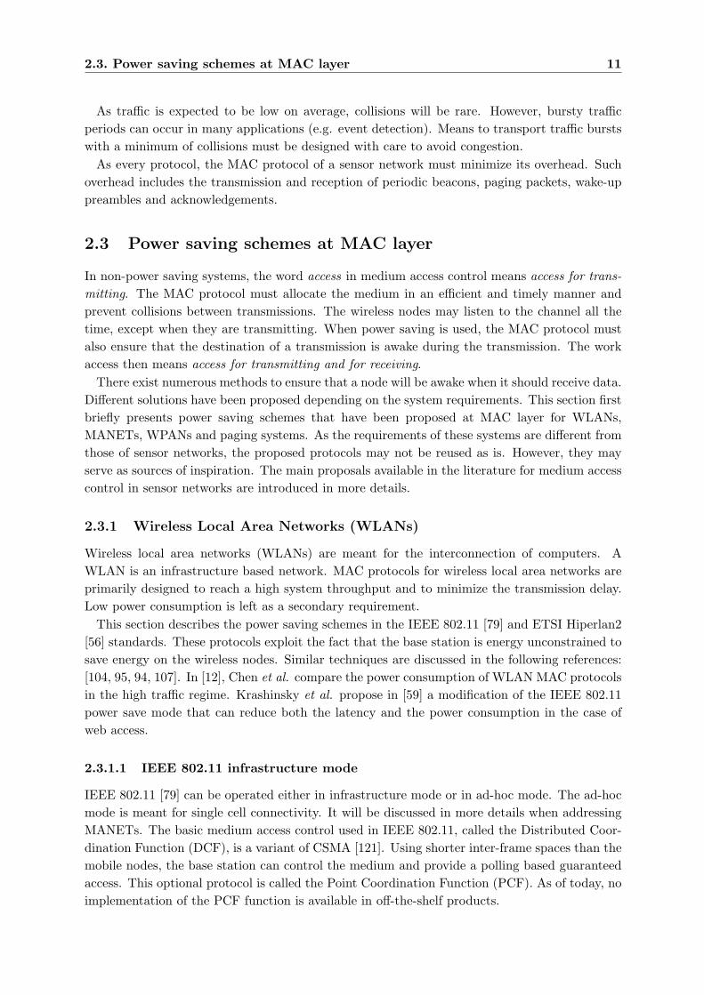
The power saving mode is based on the definition of a time window following the beaconduring which all nodes have to be awake. Transmission towards nodes in power saving modemust be announced using ATIM packets (announcement traffic indication map) sent during theso-called ATIM window. Unicast ATIM packets are acknowledged. If a power saving node hasreceived an ATIM packet announcing a broadcast packet or an unicast packet addressed to itself,it must remain awake for the full beacon interval to receive the data. Otherwise, it may go backto sleep. This procedure is illustrated in Fig. 2.2.
Several researchers have proposed enhancements to the IEEE 802.11 ad-hoc power-save mode.Woesner et al. study in [121] the trade-off between power consumption and the achievablethroughput in the choice of the duration of the ATIM window. Variants designed specificallyfor multi-hop networks are presented in [115]. The scalability of the synchronization mechanismbased on the distributed beacon generation in a multi-hop network is studied in [47].
14 Chapter 2. Energy Efficient Medium Access Control - State of the Art
576 alternating bits1010101010 ...
batch 1 batch 2 batch n
SYNC Frame 0 Frame 1 Frame 2 Frame 3 Frame 4 Frame 5 Frame 7 Frame 8
32 bits 64 bits
Figure 2.3: POCSAG paging system frame format.
2.3.2.2 Hiperlan 1
The Hiperlan 1 standard was published by ETSI in year 1996 [34]. Hiperlan 1 uses a distributedmedium access control based on a variant of CSMA called EY-NPMA (Elimination Yield - Non-Preemptive Priority Multiple Access) [121]. Hiperlan was designed to provide ad-hoc multi-hopconnectivity to mobile computers. It does not rely on a wired network infrastructure. Multi-hop communication is achieved via nodes that have taken the role of forwarders. The powersaving scheme defined in Hiperlan 1 is based on a contract between two nodes: a p-saver anda p-supporter. The p-saver is active only during periodic intervals. The p-supporter must storepackets destined to the p-saver and transmit them during the active intervals of the p-saver. Inpractice, as forwarders and p-savers will consume more energy that other nodes, it is likely thatthey will need to be powered from the mains.
Another interesting power saving scheme can be found in the framing. At high bit rate, anHiperlan 1 transceiver needs to use a power hungry equalizer. Packets start at low bit rate witha 34 bits header that can be demodulated without equalizer. This header contains an 8 bits hashof the destination address. If a node has a matching hash, it starts the equalizer and receivesthe rest of the message. With this scheme, only 1/256 = 0.4% of nodes will overhear packets.
2.3.3 Paging systems
The goal of paging systems is to minimize the power consumption on the pagers and to maxi-mizing the throughput. Latency is secondary.
2.3.3.1 POCSAG
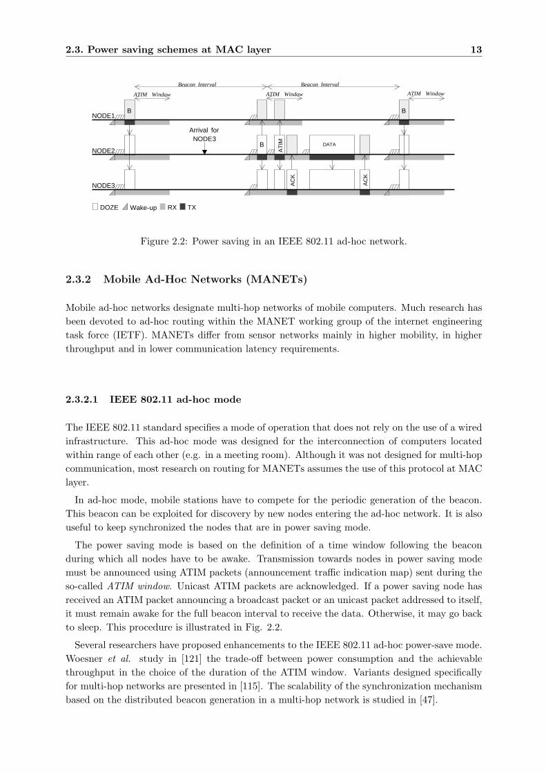
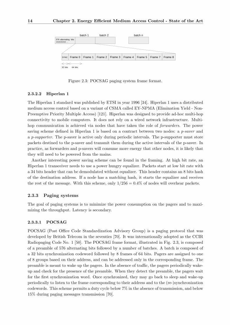
POCSAG (Post Office Code Standardization Advisory Group) is a paging protocol that wasdeveloped by British Telecom in the seventies [70]. It was internationally adopted as the CCIRRadiopaging Code No. 1 [50]. The POCSAG frame format, illustrated in Fig. 2.3, is composedof a preamble of 576 alternating bits followed by a number of batches. A batch is composed ofa 32 bits synchronization codeword followed by 8 frames of 64 bits. Pagers are assigned to oneof 8 groups based on their address, and can be addressed only in the corresponding frame. Thepreamble is meant to wake up the pagers. In the absence of traffic, the pagers periodically wake-up and check for the presence of the preamble. When they detect the preamble, the pagers waitfor the first synchronization word. Once synchronized, they may go back to sleep and wake-upperiodically to listen to the frame corresponding to their address and to the (re-)synchronizationcodewords. This scheme permits a duty cycle below 7% in the absence of transmission, and below15% during paging messages transmission [70].
2.3. Power saving schemes at MAC layer 15
2.3.3.2 FLEX and ERMES
In the beginning of the nineties, Motorola has introduced the FLEX protocol [70]. With theMotorola FLEX protocol, pagers remain continuously synchronized. A pager has to wake upevery 30 seconds to listen to the frame corresponding to its address. The addresses of all nodesfor which a message is scheduled are grouped at the beginning of the batches, allowing pagersfor which no traffic is present to quickly go back to sleep.
In Europe, the European Radio Message System (ERMES) standard was specified by ETSIas a successor to POCSAG [33]. It uses a similar approach as FLEX (keeping the networksynchronized and providing long sleep intervals). An improvement over FLEX found in ERMESconsists in sorting the addresses. This allows the pagers to go back to sleep on average afterhalf the duration of the address list.
2.3.4 Wireless Personal Area Networks (WPANs)
Wireless personal area networks (WPANs) designate short range networks centered around aperson. WPANs differ from WLANs through the increased importance of the low power con-sumption and more modest requirements in terms of throughput. The two most importantstandards for WPANs are Bluetooth [102] and IEEE 802.15.4 [82]. Both are based on a startopology, where a central node is in charge of network coordination. Because network coordina-tion requires additional energy, it can be expected that such networks will be centered aroundrechargeable devices such as mobile phones or portable computers.
2.3.4.1 Bluetooth
Bluetooth is a digital wireless data transmission standard in the 2.4 GHz ISM band aimed atproviding a short range wireless link between laptops, cellular phones and other devices [102].The air interface modulation is Gaussian FSK with a raw bit rate of 1 Mb/s (3 Mb/s in the nextversion). The communication topology between Bluetooth nodes is point-to-multipoint, wherea master communicates in time division duplex with several slaves using the polling protocol,forming a so-called piconet. In order to tolerate interference which can readily arise in the 2.4GHz band, a slow frequency hopping scheme is used, where all nodes of a piconet hop togetheramong 79 frequencies at each packet slot.
Bluetooth defines three power saving modes: hold, sniff and park. In the hold mode, the nodeleaves the piconet for an agreed period of time, possibly to save power, but also to discoveror connect to other nodes. In sniff mode, a node periodically wakes up to receive potentialtraffic. In park mode, a node leaves the piconet but remains synchronized with the hoppingsequence such that it may join the piconet rapidly once necessary. It must periodically wake upto refresh the synchronization. The piconet master, being in control of everything, may simplysleep whenever it has nothing to do.
The use of Bluetooth for multi-hop networking is possible, as a node may simultaneouslybe part of multiple piconets. This however places severe constraints in the operation of therespective piconets. Several research groups have experiments multi-hop networking based onBluetooth [55, 62]. The main drawback of Bluetooth for ad-hoc networks is the long time that isneeded to discover neighbors and connect to them. This high latency is caused by the use of thefrequency hopping technique. Bluetooth specifies that a device that wants to be discoverablelistens during 10 ms on a fixed frequency every 1.28 seconds. A different channel, chosen from 32
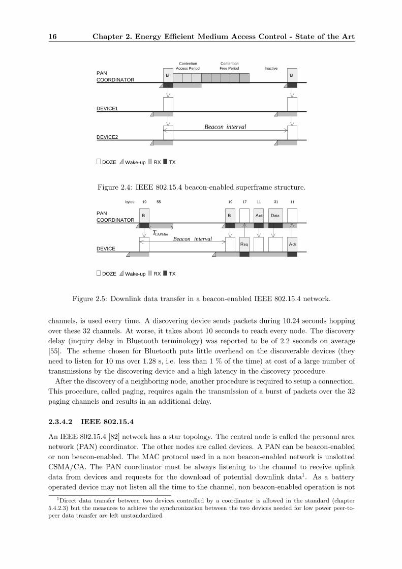
16 Chapter 2. Energy Efficient Medium Access Control - State of the Art
PANCOORDINATOR
DEVICE1
B
Wake-up TXRXDOZE
ContentionAccess Period
ContentionFree Period
DEVICE2
B
Inactive
Beacon interval
Figure 2.4: IEEE 802.15.4 beacon-enabled superframe structure.
PANCOORDINATOR
DEVICE
B
Wake-up TXRXDOZE
bytes:
TCAPMin
19 55 19
Req
Data
17 31
Ack
11
B Ack
11
Beacon interval
Figure 2.5: Downlink data transfer in a beacon-enabled IEEE 802.15.4 network.
channels, is used every time. A discovering device sends packets during 10.24 seconds hoppingover these 32 channels. At worse, it takes about 10 seconds to reach every node. The discoverydelay (inquiry delay in Bluetooth terminology) was reported to be of 2.2 seconds on average[55]. The scheme chosen for Bluetooth puts little overhead on the discoverable devices (theyneed to listen for 10 ms over 1.28 s, i.e. less than 1 % of the time) at cost of a large number oftransmissions by the discovering device and a high latency in the discovery procedure.
After the discovery of a neighboring node, another procedure is required to setup a connection.This procedure, called paging, requires again the transmission of a burst of packets over the 32paging channels and results in an additional delay.
2.3.4.2 IEEE 802.15.4
An IEEE 802.15.4 [82] network has a star topology. The central node is called the personal areanetwork (PAN) coordinator. The other nodes are called devices. A PAN can be beacon-enabledor non beacon-enabled. The MAC protocol used in a non beacon-enabled network is unslottedCSMA/CA. The PAN coordinator must be always listening to the channel to receive uplinkdata from devices and requests for the download of potential downlink data1. As a batteryoperated device may not listen all the time to the channel, non beacon-enabled operation is not
1Direct data transfer between two devices controlled by a coordinator is allowed in the standard (chapter5.4.2.3) but the measures to achieve the synchronization between the two devices needed for low power peer-to-peer data transfer are left unstandardized.
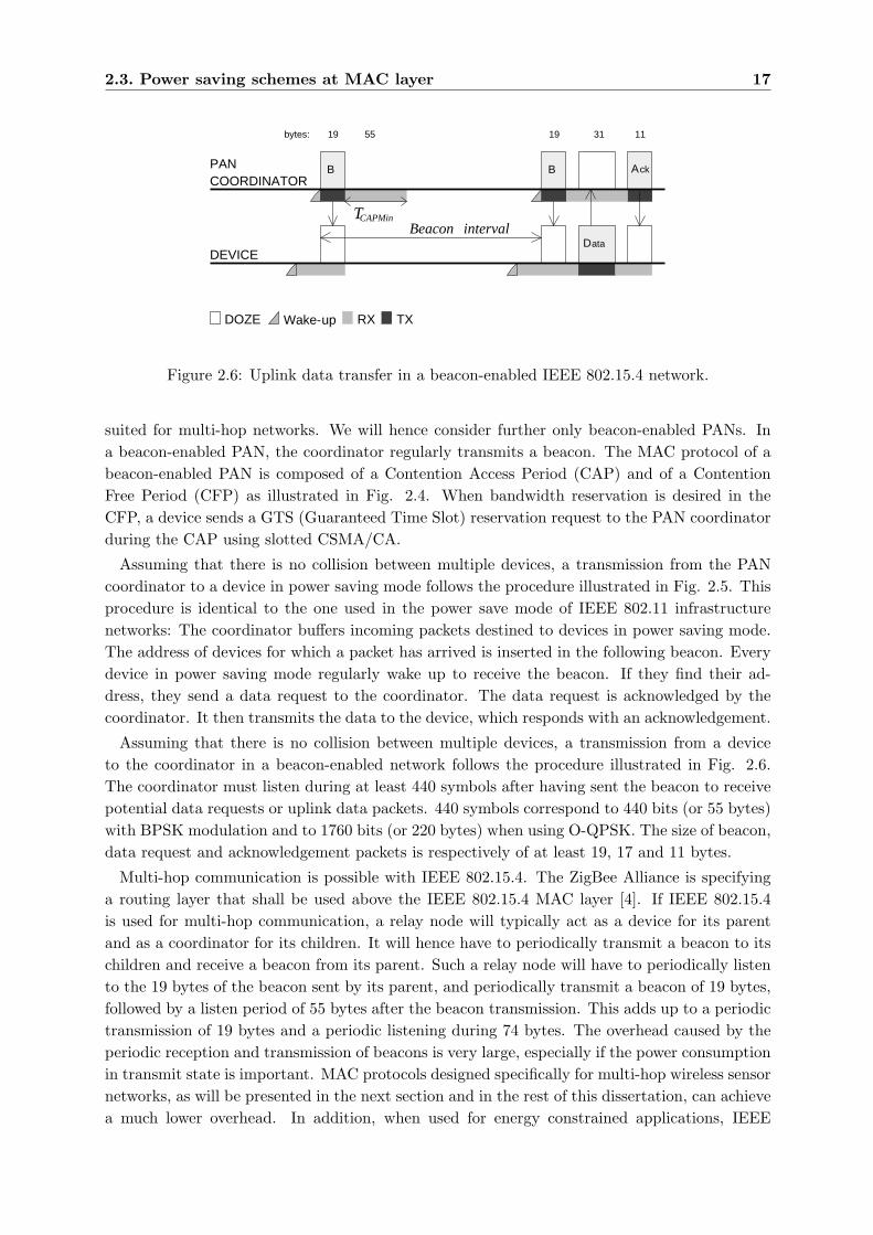
2.3. Power saving schemes at MAC layer 17
PANCOORDINATOR
DEVICE
B
Wake-up TXRXDOZE
bytes:
TCAPMin
19 55 19
Data
31
Ack
11
B
Beacon interval
Figure 2.6: Uplink data transfer in a beacon-enabled IEEE 802.15.4 network.
suited for multi-hop networks. We will hence consider further only beacon-enabled PANs. Ina beacon-enabled PAN, the coordinator regularly transmits a beacon. The MAC protocol of abeacon-enabled PAN is composed of a Contention Access Period (CAP) and of a ContentionFree Period (CFP) as illustrated in Fig. 2.4. When bandwidth reservation is desired in theCFP, a device sends a GTS (Guaranteed Time Slot) reservation request to the PAN coordinatorduring the CAP using slotted CSMA/CA.
Assuming that there is no collision between multiple devices, a transmission from the PANcoordinator to a device in power saving mode follows the procedure illustrated in Fig. 2.5. Thisprocedure is identical to the one used in the power save mode of IEEE 802.11 infrastructurenetworks: The coordinator buffers incoming packets destined to devices in power saving mode.The address of devices for which a packet has arrived is inserted in the following beacon. Everydevice in power saving mode regularly wake up to receive the beacon. If they find their ad-dress, they send a data request to the coordinator. The data request is acknowledged by thecoordinator. It then transmits the data to the device, which responds with an acknowledgement.
Assuming that there is no collision between multiple devices, a transmission from a deviceto the coordinator in a beacon-enabled network follows the procedure illustrated in Fig. 2.6.The coordinator must listen during at least 440 symbols after having sent the beacon to receivepotential data requests or uplink data packets. 440 symbols correspond to 440 bits (or 55 bytes)with BPSK modulation and to 1760 bits (or 220 bytes) when using O-QPSK. The size of beacon,data request and acknowledgement packets is respectively of at least 19, 17 and 11 bytes.
Multi-hop communication is possible with IEEE 802.15.4. The ZigBee Alliance is specifyinga routing layer that shall be used above the IEEE 802.15.4 MAC layer [4]. If IEEE 802.15.4is used for multi-hop communication, a relay node will typically act as a device for its parentand as a coordinator for its children. It will hence have to periodically transmit a beacon to itschildren and receive a beacon from its parent. Such a relay node will have to periodically listento the 19 bytes of the beacon sent by its parent, and periodically transmit a beacon of 19 bytes,followed by a listen period of 55 bytes after the beacon transmission. This adds up to a periodictransmission of 19 bytes and a periodic listening during 74 bytes. The overhead caused by theperiodic reception and transmission of beacons is very large, especially if the power consumptionin transmit state is important. MAC protocols designed specifically for multi-hop wireless sensornetworks, as will be presented in the next section and in the rest of this dissertation, can achievea much lower overhead. In addition, when used for energy constrained applications, IEEE
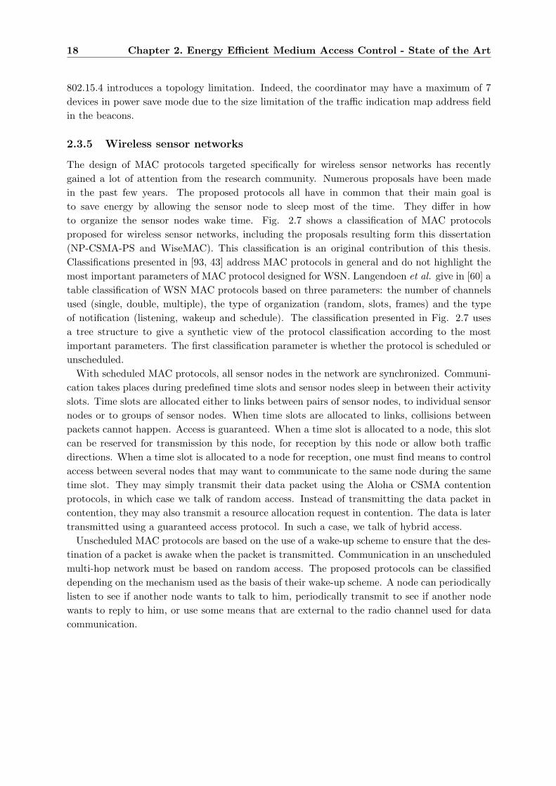
18 Chapter 2. Energy Efficient Medium Access Control - State of the Art
802.15.4 introduces a topology limitation. Indeed, the coordinator may have a maximum of 7devices in power save mode due to the size limitation of the traffic indication map address fieldin the beacons.
2.3.5 Wireless sensor networks
The design of MAC protocols targeted specifically for wireless sensor networks has recentlygained a lot of attention from the research community. Numerous proposals have been madein the past few years. The proposed protocols all have in common that their main goal isto save energy by allowing the sensor node to sleep most of the time. They differ in howto organize the sensor nodes wake time. Fig. 2.7 shows a classification of MAC protocolsproposed for wireless sensor networks, including the proposals resulting form this dissertation(NP-CSMA-PS and WiseMAC). This classification is an original contribution of this thesis.Classifications presented in [93, 43] address MAC protocols in general and do not highlight themost important parameters of MAC protocol designed for WSN. Langendoen et al. give in [60] atable classification of WSN MAC protocols based on three parameters: the number of channelsused (single, double, multiple), the type of organization (random, slots, frames) and the typeof notification (listening, wakeup and schedule). The classification presented in Fig. 2.7 usesa tree structure to give a synthetic view of the protocol classification according to the mostimportant parameters. The first classification parameter is whether the protocol is scheduled orunscheduled.
With scheduled MAC protocols, all sensor nodes in the network are synchronized. Communi-cation takes places during predefined time slots and sensor nodes sleep in between their activityslots. Time slots are allocated either to links between pairs of sensor nodes, to individual sensornodes or to groups of sensor nodes. When time slots are allocated to links, collisions betweenpackets cannot happen. Access is guaranteed. When a time slot is allocated to a node, this slotcan be reserved for transmission by this node, for reception by this node or allow both trafficdirections. When a time slot is allocated to a node for reception, one must find means to controlaccess between several nodes that may want to communicate to the same node during the sametime slot. They may simply transmit their data packet using the Aloha or CSMA contentionprotocols, in which case we talk of random access. Instead of transmitting the data packet incontention, they may also transmit a resource allocation request in contention. The data is latertransmitted using a guaranteed access protocol. In such a case, we talk of hybrid access.
Unscheduled MAC protocols are based on the use of a wake-up scheme to ensure that the des-tination of a packet is awake when the packet is transmitted. Communication in an unscheduledmulti-hop network must be based on random access. The proposed protocols can be classifieddepending on the mechanism used as the basis of their wake-up scheme. A node can periodicallylisten to see if another node wants to talk to him, periodically transmit to see if another nodewants to reply to him, or use some means that are external to the radio channel used for datacommunication.
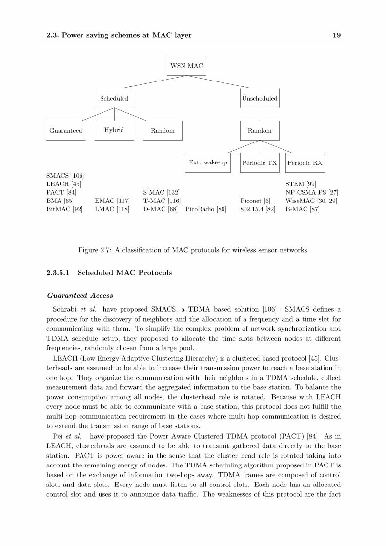
2.3. Power saving schemes at MAC layer 19
WSN MACÃÃÃÃÃÃÃÃÃÃ
`````````
Scheduled
!!!!!
aaaaa
Unscheduled
Guaranteed
SMACS [106]LEACH [45]PACT [84]BMA [65]BitMAC [92]
Hybrid
EMAC [117]LMAC [118]
Random
S-MAC [132]T-MAC [116]D-MAC [68]
Random
!!!!!
aaaaa
Ext. wake-up
PicoRadio [89]
Periodic TX
Piconet [6]802.15.4 [82]
Periodic RX
STEM [99]NP-CSMA-PS [27]WiseMAC [30, 29]B-MAC [87]
Figure 2.7: A classification of MAC protocols for wireless sensor networks.
2.3.5.1 Scheduled MAC Protocols
Guaranteed Access
Sohrabi et al. have proposed SMACS, a TDMA based solution [106]. SMACS defines aprocedure for the discovery of neighbors and the allocation of a frequency and a time slot forcommunicating with them. To simplify the complex problem of network synchronization andTDMA schedule setup, they proposed to allocate the time slots between nodes at differentfrequencies, randomly chosen from a large pool.
LEACH (Low Energy Adaptive Clustering Hierarchy) is a clustered based protocol [45]. Clus-terheads are assumed to be able to increase their transmission power to reach a base station inone hop. They organize the communication with their neighbors in a TDMA schedule, collectmeasurement data and forward the aggregated information to the base station. To balance thepower consumption among all nodes, the clusterhead role is rotated. Because with LEACHevery node must be able to communicate with a base station, this protocol does not fulfill themulti-hop communication requirement in the cases where multi-hop communication is desiredto extend the transmission range of base stations.
Pei et al. have proposed the Power Aware Clustered TDMA protocol (PACT) [84]. As inLEACH, clusterheads are assumed to be able to transmit gathered data directly to the basestation. PACT is power aware in the sense that the cluster head role is rotated taking intoaccount the remaining energy of nodes. The TDMA scheduling algorithm proposed in PACT isbased on the exchange of information two-hops away. TDMA frames are composed of controlslots and data slots. Every node must listen to all control slots. Each node has an allocatedcontrol slot and uses it to announce data traffic. The weaknesses of this protocol are the fact
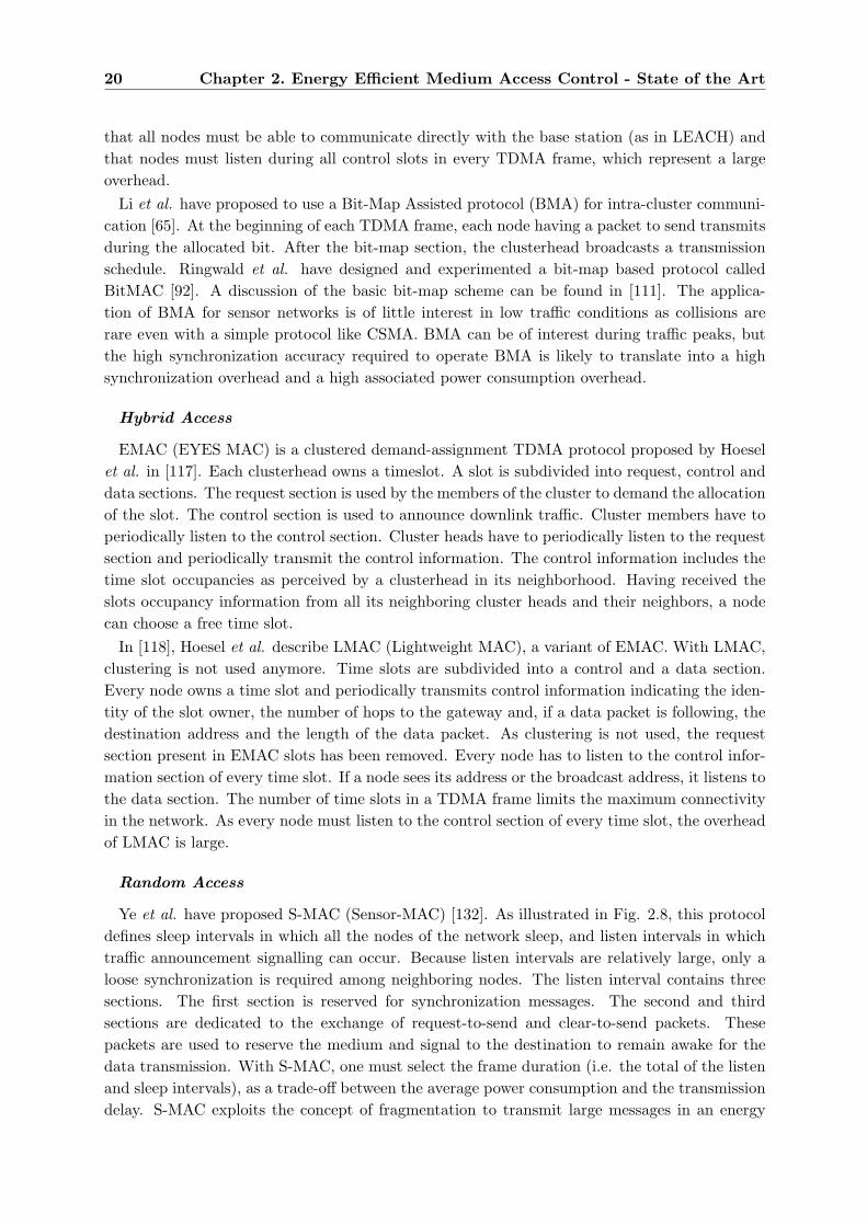
20 Chapter 2. Energy Efficient Medium Access Control - State of the Art
that all nodes must be able to communicate directly with the base station (as in LEACH) andthat nodes must listen during all control slots in every TDMA frame, which represent a largeoverhead.
Li et al. have proposed to use a Bit-Map Assisted protocol (BMA) for intra-cluster communi-cation [65]. At the beginning of each TDMA frame, each node having a packet to send transmitsduring the allocated bit. After the bit-map section, the clusterhead broadcasts a transmissionschedule. Ringwald et al. have designed and experimented a bit-map based protocol calledBitMAC [92]. A discussion of the basic bit-map scheme can be found in [111]. The applica-tion of BMA for sensor networks is of little interest in low traffic conditions as collisions arerare even with a simple protocol like CSMA. BMA can be of interest during traffic peaks, butthe high synchronization accuracy required to operate BMA is likely to translate into a highsynchronization overhead and a high associated power consumption overhead.
Hybrid Access
EMAC (EYES MAC) is a clustered demand-assignment TDMA protocol proposed by Hoeselet al. in [117]. Each clusterhead owns a timeslot. A slot is subdivided into request, control anddata sections. The request section is used by the members of the cluster to demand the allocationof the slot. The control section is used to announce downlink traffic. Cluster members have toperiodically listen to the control section. Cluster heads have to periodically listen to the requestsection and periodically transmit the control information. The control information includes thetime slot occupancies as perceived by a clusterhead in its neighborhood. Having received theslots occupancy information from all its neighboring cluster heads and their neighbors, a nodecan choose a free time slot.
In [118], Hoesel et al. describe LMAC (Lightweight MAC), a variant of EMAC. With LMAC,clustering is not used anymore. Time slots are subdivided into a control and a data section.Every node owns a time slot and periodically transmits control information indicating the iden-tity of the slot owner, the number of hops to the gateway and, if a data packet is following, thedestination address and the length of the data packet. As clustering is not used, the requestsection present in EMAC slots has been removed. Every node has to listen to the control infor-mation section of every time slot. If a node sees its address or the broadcast address, it listens tothe data section. The number of time slots in a TDMA frame limits the maximum connectivityin the network. As every node must listen to the control section of every time slot, the overheadof LMAC is large.
Random Access
Ye et al. have proposed S-MAC (Sensor-MAC) [132]. As illustrated in Fig. 2.8, this protocoldefines sleep intervals in which all the nodes of the network sleep, and listen intervals in whichtraffic announcement signalling can occur. Because listen intervals are relatively large, only aloose synchronization is required among neighboring nodes. The listen interval contains threesections. The first section is reserved for synchronization messages. The second and thirdsections are dedicated to the exchange of request-to-send and clear-to-send packets. Thesepackets are used to reserve the medium and signal to the destination to remain awake for thedata transmission. With S-MAC, one must select the frame duration (i.e. the total of the listenand sleep intervals), as a trade-off between the average power consumption and the transmissiondelay. S-MAC exploits the concept of fragmentation to transmit large messages in an energy
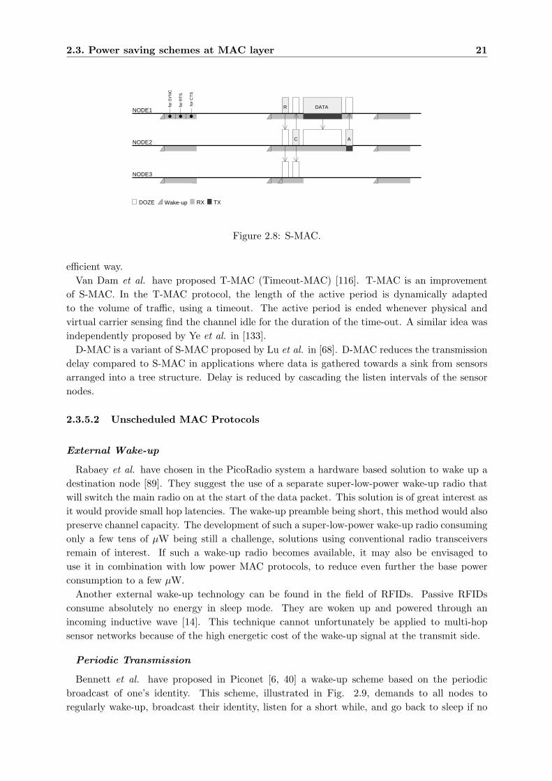
2.3. Power saving schemes at MAC layer 21
NODE1
NODE2
Wake-up TXRXDOZE
NODE3
R
C
DATA
A
for
SY
NC
for
RT
S
for
CT
S
Figure 2.8: S-MAC.
efficient way.Van Dam et al. have proposed T-MAC (Timeout-MAC) [116]. T-MAC is an improvement
of S-MAC. In the T-MAC protocol, the length of the active period is dynamically adaptedto the volume of traffic, using a timeout. The active period is ended whenever physical andvirtual carrier sensing find the channel idle for the duration of the time-out. A similar idea wasindependently proposed by Ye et al. in [133].
D-MAC is a variant of S-MAC proposed by Lu et al. in [68]. D-MAC reduces the transmissiondelay compared to S-MAC in applications where data is gathered towards a sink from sensorsarranged into a tree structure. Delay is reduced by cascading the listen intervals of the sensornodes.
2.3.5.2 Unscheduled MAC Protocols
External Wake-up
Rabaey et al. have chosen in the PicoRadio system a hardware based solution to wake up adestination node [89]. They suggest the use of a separate super-low-power wake-up radio thatwill switch the main radio on at the start of the data packet. This solution is of great interest asit would provide small hop latencies. The wake-up preamble being short, this method would alsopreserve channel capacity. The development of such a super-low-power wake-up radio consumingonly a few tens of µW being still a challenge, solutions using conventional radio transceiversremain of interest. If such a wake-up radio becomes available, it may also be envisaged touse it in combination with low power MAC protocols, to reduce even further the base powerconsumption to a few µW.
Another external wake-up technology can be found in the field of RFIDs. Passive RFIDsconsume absolutely no energy in sleep mode. They are woken up and powered through anincoming inductive wave [14]. This technique cannot unfortunately be applied to multi-hopsensor networks because of the high energetic cost of the wake-up signal at the transmit side.
Periodic Transmission
Bennett et al. have proposed in Piconet [6, 40] a wake-up scheme based on the periodicbroadcast of one’s identity. This scheme, illustrated in Fig. 2.9, demands to all nodes toregularly wake-up, broadcast their identity, listen for a short while, and go back to sleep if no
22 Chapter 2. Energy Efficient Medium Access Control - State of the Art
ID
NODE1
NODE2
Wake-up TXRXDOZE
NODE3
DATA
AID
ID
ID ID
ID
Figure 2.9: Piconet.
data reception has started. This approach can provide very low power consumption when littletraffic is present and when the wake-up interval is large. Data packets are sent when the intendeddestination is listening. At that time, having a very low duty cycle, the other neighboring nodesare very likely to sleep. Hence, this protocol provides a solution to the problem of overhearing.Limitations of this protocol appear when a wake-up interval in the order of 100 ms is desiredin order to have a short hop transmission delay. The first problem is then that the backgroundtraffic caused by the broadcast of the ID packets becomes non-negligible and can cause frequentcollisions with data packets. Secondly, the average power needed to transmit the ID packet andto listen for potential replies becomes important. Note finally that the periodic ID broadcast inPiconet is similar to the periodic beacon transmission in IEEE 802.15.4.
Periodic Listening
Schurgers et al. have proposed STEM [99]. This protocol uses two channels: one pagingchannel and one traffic channel. Most of the time, the network is expected to be in the monitoringstate, and only the paging channel is used. In case of an alarm, for example, a path on thedata channel is opened throughout the network, where communication occurs using a regularwireless protocol (not low power). In STEM, the paging channel is implemented at the receiverside by regularly listening to the channel during the time needed to receive a paging packet. Atransmitter that wants to page one of its neighbor will repeat a paging packet containing thedestination address, until a reply is received. The operation of the paging channel is illustrated inFig. 2.10. This protocol provides a low power consumption in the absence of traffic, the pagingchannel consuming little energy. The weakness of this protocol is mainly its inefficiency totransport small amount of periodic or sporadic traffic. Note that the wake-up scheme proposedby STEM can be seen as a simplified version, at a single frequency, of the discovery procedureused in Bluetooth.
NP-CSMA-PS [26, 27] and WiseMAC [30, 29] are proposals resulting from this dissertation.They will be discussed in the following chapters.
B-MAC is a CSMA based protocol. It has been developed at Berkeley and implementedon TinyOS [109]. To reduce the idle listening power consumption, B-MAC uses the preamblesampling technique described in [26]. In the context of B-MAC, preamble sampling is called LowPower Listening (LPL). The particularity of B-MAC is to have been implemented on TinyOSwith a rich configuration interface, allowing the application programmer to configure the protocolmechanisms (clear channel assessment, acknowledgements, backoffs and LPL).
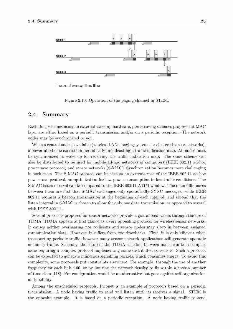
2.4. Summary 23
B B B
A
NODE1
NODE2
Wake-up TXRXDOZE
NODE3
A
B B B
Figure 2.10: Operation of the paging channel in STEM.
2.4 Summary
Excluding schemes using an external wake-up hardware, power saving schemes proposed at MAClayer are either based on a periodic transmission and/or on a periodic reception. The networknodes may be synchronized or not.
When a central node is available (wireless LANs, paging systems, or clustered sensor networks),a powerful scheme consists in periodically broadcasting a traffic indication map. All nodes mustbe synchronized to wake up for receiving the traffic indication map. The same scheme canalso be distributed to be used for mobile ad-hoc networks of computers (IEEE 802.11 ad-hocpower save protocol) and sensor networks (S-MAC). Synchronization becomes more challengingin such cases. The S-MAC protocol can be seen as an extreme case of the IEEE 802.11 ad-hocpower save protocol, an optimization for low power consumption in low traffic conditions. TheS-MAC listen interval can be compared to the IEEE 802.11 ATIM window. The main differencesbetween them are first that S-MAC exchanges only sporadically SYNC messages, while IEEE802.11 requires a beacon transmission at the beginning of each interval, and second that thelisten interval in S-MAC is chosen to allow for only one data transmission, as opposed to severalwith IEEE 802.11.
Several protocols proposed for sensor networks provide a guaranteed access through the use ofTDMA. TDMA appears at first glance as a very appealing protocol for wireless sensor networks.It causes neither overhearing nor collisions and sensor nodes may sleep in between assignedcommunication slots. However, it suffers from two drawbacks. First, it is only efficient whentransporting periodic traffic, however many sensor network applications will generate sporadicor bursty traffic. Secondly, the setup of the TDMA schedule between nodes can be a complexissue requiring a complex protocol implementing some distributed consensus. Such a protocolcan be expected to generate numerous signalling packets, which consumes energy. To avoid thiscomplexity, some proposals put constraints elsewhere. For example, through the use of anotherfrequency for each link [106] or by limiting the network density to fit within a chosen numberof time slots [118]. Pre-configuration would be an alternative but goes against self-organizationand mobility.
Among the unscheduled protocols, Piconet is an example of protocols based on a periodictransmission. A node having traffic to send will listen until its receives a signal. STEM isthe opposite example. It is based on a periodic reception. A node having traffic to send
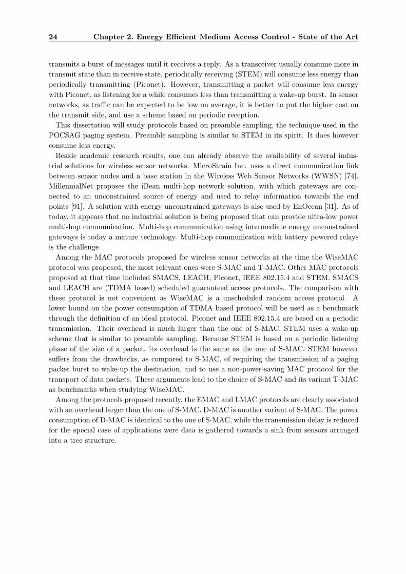
24 Chapter 2. Energy Efficient Medium Access Control - State of the Art
transmits a burst of messages until it receives a reply. As a transceiver usually consume more intransmit state than in receive state, periodically receiving (STEM) will consume less energy thanperiodically transmitting (Piconet). However, transmitting a packet will consume less energywith Piconet, as listening for a while consumes less than transmitting a wake-up burst. In sensornetworks, as traffic can be expected to be low on average, it is better to put the higher cost onthe transmit side, and use a scheme based on periodic reception.
This dissertation will study protocols based on preamble sampling, the technique used in thePOCSAG paging system. Preamble sampling is similar to STEM in its spirit. It does howeverconsume less energy.
Beside academic research results, one can already observe the availability of several indus-trial solutions for wireless sensor networks. MicroStrain Inc. uses a direct communication linkbetween sensor nodes and a base station in the Wireless Web Sensor Networks (WWSN) [74].MillennialNet proposes the iBean multi-hop network solution, with which gateways are con-nected to an unconstrained source of energy and used to relay information towards the endpoints [91]. A solution with energy unconstrained gateways is also used by EnOcean [31]. As oftoday, it appears that no industrial solution is being proposed that can provide ultra-low powermulti-hop communication. Multi-hop communication using intermediate energy unconstrainedgateways is today a mature technology. Multi-hop communication with battery powered relaysis the challenge.
Among the MAC protocols proposed for wireless sensor networks at the time the WiseMACprotocol was proposed, the most relevant ones were S-MAC and T-MAC. Other MAC protocolsproposed at that time included SMACS, LEACH, Piconet, IEEE 802.15.4 and STEM. SMACSand LEACH are (TDMA based) scheduled guaranteed access protocols. The comparison withthese protocol is not convenient as WiseMAC is a unscheduled random access protocol. Alower bound on the power consumption of TDMA based protocol will be used as a benchmarkthrough the definition of an ideal protocol. Piconet and IEEE 802.15.4 are based on a periodictransmission. Their overhead is much larger than the one of S-MAC. STEM uses a wake-upscheme that is similar to preamble sampling. Because STEM is based on a periodic listeningphase of the size of a packet, its overhead is the same as the one of S-MAC. STEM howeversuffers from the drawbacks, as compared to S-MAC, of requiring the transmission of a pagingpacket burst to wake-up the destination, and to use a non-power-saving MAC protocol for thetransport of data packets. These arguments lead to the choice of S-MAC and its variant T-MACas benchmarks when studying WiseMAC.
Among the protocols proposed recently, the EMAC and LMAC protocols are clearly associatedwith an overhead larger than the one of S-MAC. D-MAC is another variant of S-MAC. The powerconsumption of D-MAC is identical to the one of S-MAC, while the transmission delay is reducedfor the special case of applications were data is gathered towards a sink from sensors arrangedinto a tree structure.

Chapter 3
Battery and Transceiver Models
3.1 Introduction
To evaluate the performance of an ultra-low power medium access control protocol, one needsa very precise model of the radio transceiver power consumption. Existing models available inthe literature (e.g. [37]) did not describe the energy consumed when switching between stablestates. When the average power consumption is in the order of a few tens of microwatts, itis required to take into account the energy spent to turn the radio on and to switch betweenreceive and transmit states. Those energy amounts are not negligible anymore.
To translate an ultra-low average power consumption into a lifetime, it is required to use abattery model that takes into account the self-discharge of the battery. A simple battery modelhas been designed to evaluate the expected lifetime assuming a constant self-discharge.
Section 3.2 presents the battery model and section 3.3 the radio transceiver model.
3.2 Battery model
There exist many different energy sources that can be used for sensor network applications.Energy can be taken from a primary battery (non-rechargeable), from a secondary battery(rechargeable), or taken out of the environment (e.g. light and vibrations energy scavenging[89, 52]). Secondary batteries may be used in combination with energy scavenging to storethe excess energy production. In applications where energy scavenging is not possible or notsufficiently reliable, one must rely on primary batteries.
The two primary battery technologies that are best suited for low power wireless communica-tion applications, in terms of cost, shelf-life and delivered peak current, are alkaline and lithium.Lithium/manganese batteries provide a constant voltage of 3 V over their lifetime [22], whilealkaline batteries have a sloping discharge curve starting at 1.6 V and ending at about 1 V [21].The discharge curve for both technologies is illustrated in Fig. 3.1.
When designing battery powered systems with a target lifetime counted in years, it is im-portant to take into consideration the self-discharge. Alkaline batteries present a self-dischargeper year of several percents of their capacity, while lithium batteries loose about one percentor less [57]. For example, a Duracell alkaline battery will loose 5% of its capacity during thefirst year and 2% during the subsequent years [21]. An Energizer E91 AA alkaline battery willloose 20% of its capacity in seven years, giving a discharge rate of 3% per year [36]. In contrast,a Duracell lithium/manganese battery will loose only 3% of its capacity after 5 years, giving
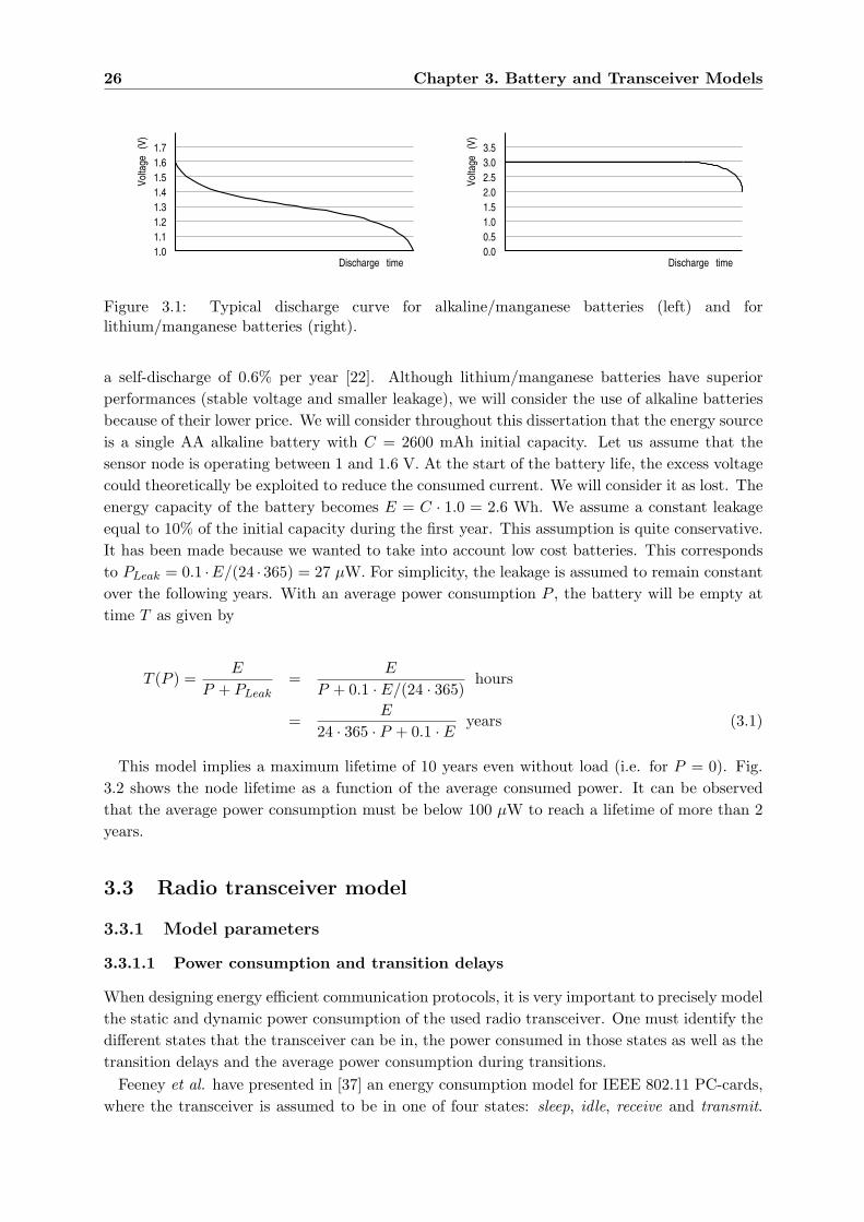
26 Chapter 3. Battery and Transceiver Models
Vol
tage
(V)
Discharge time
1.2
1.4
1.6
1.5
1.3
1.1
1.0
1.7
Vol
tage
(V)
Discharge time
1.0
2.0
3.0
2.5
1.5
0.5
0.0
3.5
Figure 3.1: Typical discharge curve for alkaline/manganese batteries (left) and forlithium/manganese batteries (right).
a self-discharge of 0.6% per year [22]. Although lithium/manganese batteries have superiorperformances (stable voltage and smaller leakage), we will consider the use of alkaline batteriesbecause of their lower price. We will consider throughout this dissertation that the energy sourceis a single AA alkaline battery with C = 2600 mAh initial capacity. Let us assume that thesensor node is operating between 1 and 1.6 V. At the start of the battery life, the excess voltagecould theoretically be exploited to reduce the consumed current. We will consider it as lost. Theenergy capacity of the battery becomes E = C · 1.0 = 2.6 Wh. We assume a constant leakageequal to 10% of the initial capacity during the first year. This assumption is quite conservative.It has been made because we wanted to take into account low cost batteries. This correspondsto PLeak = 0.1 ·E/(24 · 365) = 27 µW. For simplicity, the leakage is assumed to remain constantover the following years. With an average power consumption P , the battery will be empty attime T as given by
T (P ) =E
P + PLeak=
E
P + 0.1 · E/(24 · 365)hours
=E
24 · 365 · P + 0.1 · E years (3.1)
This model implies a maximum lifetime of 10 years even without load (i.e. for P = 0). Fig.3.2 shows the node lifetime as a function of the average consumed power. It can be observedthat the average power consumption must be below 100 µW to reach a lifetime of more than 2years.
3.3 Radio transceiver model
3.3.1 Model parameters
3.3.1.1 Power consumption and transition delays
When designing energy efficient communication protocols, it is very important to precisely modelthe static and dynamic power consumption of the used radio transceiver. One must identify thedifferent states that the transceiver can be in, the power consumed in those states as well as thetransition delays and the average power consumption during transitions.
Feeney et al. have presented in [37] an energy consumption model for IEEE 802.11 PC-cards,where the transceiver is assumed to be in one of four states: sleep, idle, receive and transmit.
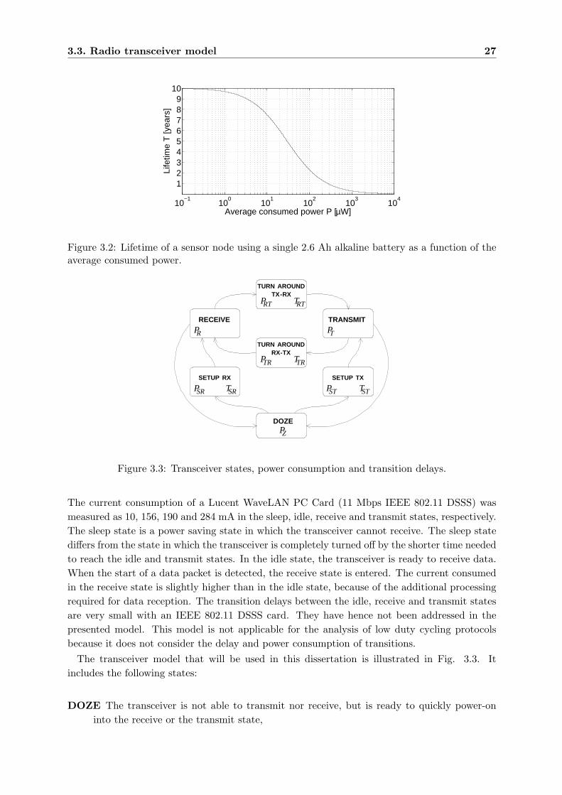
3.3. Radio transceiver model 27
10−1
100
101
102
103
104
123456789
10
Average consumed power P [µW]
Life
time
T [y
ears
]
Figure 3.2: Lifetime of a sensor node using a single 2.6 Ah alkaline battery as a function of theaverage consumed power.
PZDOZE
RECEIVE
PR
TURN AROUNDTX-RX
PRT
SETUP RX
PSR TSR
SETUP TX
PST TST
TRANSMIT
PTTURN AROUND
RX-TXPTR TTR
TRT
Figure 3.3: Transceiver states, power consumption and transition delays.
The current consumption of a Lucent WaveLAN PC Card (11 Mbps IEEE 802.11 DSSS) wasmeasured as 10, 156, 190 and 284 mA in the sleep, idle, receive and transmit states, respectively.The sleep state is a power saving state in which the transceiver cannot receive. The sleep statediffers from the state in which the transceiver is completely turned off by the shorter time neededto reach the idle and transmit states. In the idle state, the transceiver is ready to receive data.When the start of a data packet is detected, the receive state is entered. The current consumedin the receive state is slightly higher than in the idle state, because of the additional processingrequired for data reception. The transition delays between the idle, receive and transmit statesare very small with an IEEE 802.11 DSSS card. They have hence not been addressed in thepresented model. This model is not applicable for the analysis of low duty cycling protocolsbecause it does not consider the delay and power consumption of transitions.
The transceiver model that will be used in this dissertation is illustrated in Fig. 3.3. Itincludes the following states:
DOZE The transceiver is not able to transmit nor receive, but is ready to quickly power-oninto the receive or the transmit state,
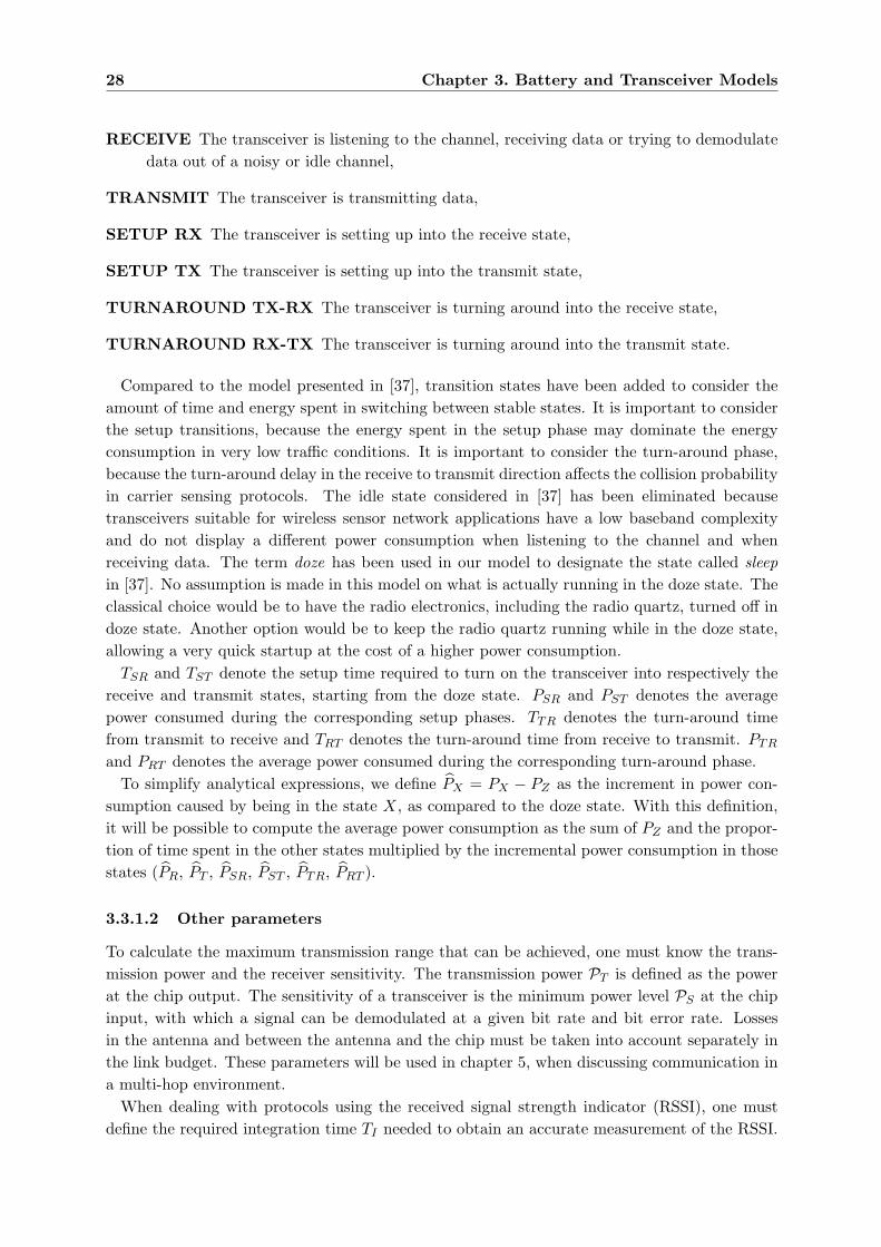
28 Chapter 3. Battery and Transceiver Models
RECEIVE The transceiver is listening to the channel, receiving data or trying to demodulatedata out of a noisy or idle channel,
TRANSMIT The transceiver is transmitting data,
SETUP RX The transceiver is setting up into the receive state,
SETUP TX The transceiver is setting up into the transmit state,
TURNAROUND TX-RX The transceiver is turning around into the receive state,
TURNAROUND RX-TX The transceiver is turning around into the transmit state.
Compared to the model presented in [37], transition states have been added to consider theamount of time and energy spent in switching between stable states. It is important to considerthe setup transitions, because the energy spent in the setup phase may dominate the energyconsumption in very low traffic conditions. It is important to consider the turn-around phase,because the turn-around delay in the receive to transmit direction affects the collision probabilityin carrier sensing protocols. The idle state considered in [37] has been eliminated becausetransceivers suitable for wireless sensor network applications have a low baseband complexityand do not display a different power consumption when listening to the channel and whenreceiving data. The term doze has been used in our model to designate the state called sleepin [37]. No assumption is made in this model on what is actually running in the doze state. Theclassical choice would be to have the radio electronics, including the radio quartz, turned off indoze state. Another option would be to keep the radio quartz running while in the doze state,allowing a very quick startup at the cost of a higher power consumption.
TSR and TST denote the setup time required to turn on the transceiver into respectively thereceive and transmit states, starting from the doze state. PSR and PST denotes the averagepower consumed during the corresponding setup phases. TTR denotes the turn-around timefrom transmit to receive and TRT denotes the turn-around time from receive to transmit. PTR
and PRT denotes the average power consumed during the corresponding turn-around phase.To simplify analytical expressions, we define PX = PX − PZ as the increment in power con-
sumption caused by being in the state X, as compared to the doze state. With this definition,it will be possible to compute the average power consumption as the sum of PZ and the propor-tion of time spent in the other states multiplied by the incremental power consumption in thosestates (PR, PT , PSR, PST , PTR, PRT ).
3.3.1.2 Other parameters
To calculate the maximum transmission range that can be achieved, one must know the trans-mission power and the receiver sensitivity. The transmission power PT is defined as the powerat the chip output. The sensitivity of a transceiver is the minimum power level PS at the chipinput, with which a signal can be demodulated at a given bit rate and bit error rate. Lossesin the antenna and between the antenna and the chip must be taken into account separately inthe link budget. These parameters will be used in chapter 5, when discussing communication ina multi-hop environment.
When dealing with protocols using the received signal strength indicator (RSSI), one mustdefine the required integration time TI needed to obtain an accurate measurement of the RSSI.
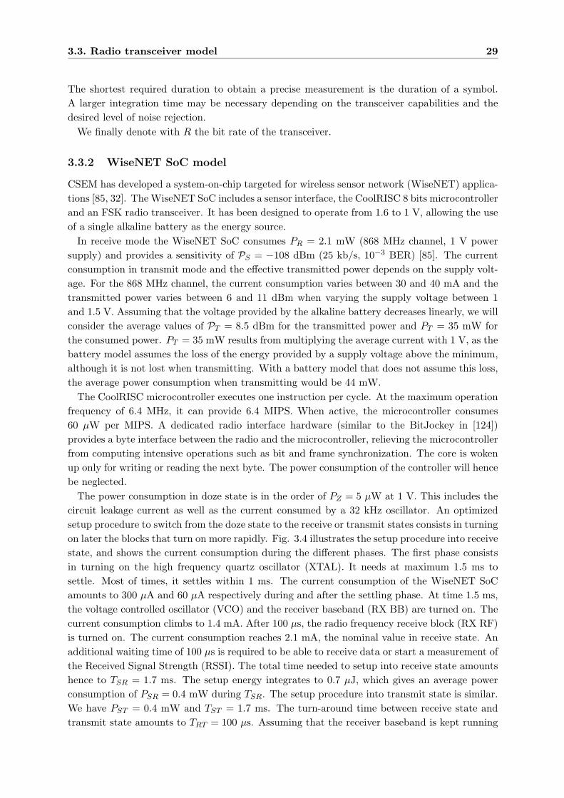
3.3. Radio transceiver model 29
The shortest required duration to obtain a precise measurement is the duration of a symbol.A larger integration time may be necessary depending on the transceiver capabilities and thedesired level of noise rejection.
We finally denote with R the bit rate of the transceiver.
3.3.2 WiseNET SoC model
CSEM has developed a system-on-chip targeted for wireless sensor network (WiseNET) applica-tions [85, 32]. The WiseNET SoC includes a sensor interface, the CoolRISC 8 bits microcontrollerand an FSK radio transceiver. It has been designed to operate from 1.6 to 1 V, allowing the useof a single alkaline battery as the energy source.
In receive mode the WiseNET SoC consumes PR = 2.1 mW (868 MHz channel, 1 V powersupply) and provides a sensitivity of PS = −108 dBm (25 kb/s, 10−3 BER) [85]. The currentconsumption in transmit mode and the effective transmitted power depends on the supply volt-age. For the 868 MHz channel, the current consumption varies between 30 and 40 mA and thetransmitted power varies between 6 and 11 dBm when varying the supply voltage between 1and 1.5 V. Assuming that the voltage provided by the alkaline battery decreases linearly, we willconsider the average values of PT = 8.5 dBm for the transmitted power and PT = 35 mW forthe consumed power. PT = 35 mW results from multiplying the average current with 1 V, as thebattery model assumes the loss of the energy provided by a supply voltage above the minimum,although it is not lost when transmitting. With a battery model that does not assume this loss,the average power consumption when transmitting would be 44 mW.
The CoolRISC microcontroller executes one instruction per cycle. At the maximum operationfrequency of 6.4 MHz, it can provide 6.4 MIPS. When active, the microcontroller consumes60 µW per MIPS. A dedicated radio interface hardware (similar to the BitJockey in [124])provides a byte interface between the radio and the microcontroller, relieving the microcontrollerfrom computing intensive operations such as bit and frame synchronization. The core is wokenup only for writing or reading the next byte. The power consumption of the controller will hencebe neglected.
The power consumption in doze state is in the order of PZ = 5 µW at 1 V. This includes thecircuit leakage current as well as the current consumed by a 32 kHz oscillator. An optimizedsetup procedure to switch from the doze state to the receive or transmit states consists in turningon later the blocks that turn on more rapidly. Fig. 3.4 illustrates the setup procedure into receivestate, and shows the current consumption during the different phases. The first phase consistsin turning on the high frequency quartz oscillator (XTAL). It needs at maximum 1.5 ms tosettle. Most of times, it settles within 1 ms. The current consumption of the WiseNET SoCamounts to 300 µA and 60 µA respectively during and after the settling phase. At time 1.5 ms,the voltage controlled oscillator (VCO) and the receiver baseband (RX BB) are turned on. Thecurrent consumption climbs to 1.4 mA. After 100 µs, the radio frequency receive block (RX RF)is turned on. The current consumption reaches 2.1 mA, the nominal value in receive state. Anadditional waiting time of 100 µs is required to be able to receive data or start a measurement ofthe Received Signal Strength (RSSI). The total time needed to setup into receive state amountshence to TSR = 1.7 ms. The setup energy integrates to 0.7 µJ, which gives an average powerconsumption of PSR = 0.4 mW during TSR. The setup procedure into transmit state is similar.We have PST = 0.4 mW and TST = 1.7 ms. The turn-around time between receive state andtransmit state amounts to TRT = 100 µs. Assuming that the receiver baseband is kept running

30 Chapter 3. Battery and Transceiver Models
Cur
rent
(mA
)
Time (ms)
2
0
1
1.5
0.5
0 10.5 1.5
XTAL On VCO and RX BB On
RX RF On
100 us
100 us
1.5 ms
Figure 3.4: Current consumption of the WiseNET SoC during setup phase into receive state.
Table 3.1: Parameters used for the WiseNET SoC model.PZ = 5 µW PSR = PS = 0.4 mW TSR = TS = 1.7 ms PT = 8.5 dBmPR = 2.1 mW PST = PS = 0.4 mW TST = TS = 1.7 ms PS = −108 dBm (BER=10−3)PT = 35 mW PTR = PR = 2.1 mW TTR = TT = 0.1 ms R = 25 kbpsU = 1.0 V PRT = PR = 2.1 mW TRT = TT = 0.1 ms TI = 100 µs
during transmit, the same value can be used for the transmit to receive turn-around time TTR.During the turn-around phases, the power consumption is assumed to be equal to the powerconsumption is receive state (PRT = PTR = PR). It is assumed to operate the transceiver atR = 25 kbps, giving a bit duration of 40 µs. To reach a reasonable accuracy when measuring thereceived signal strength, the integration time should be TI = 100 µs. As radio and controller areintegrated into a single chip, the time to read the RSSI value can be neglected. The parametersused for the WiseNET SoC model are summarized in table 3.1.
As the setup time and power consumption into receive and transmit states is identical for theWiseNET SoC, we will simplify the notation and use TS and PS instead of TSR, TST and PSR,PST respectively. As the turn-around time is equal in both directions, we will use the notationTT instead of TTR and TRT .
3.4 Conclusion
In this chapter, an alkaline battery model has been defined, assuming a constant self-dischargeequivalent to loosing 10% of the initial capacity in one year. This model can be consideredas quite conservative. Recent performance figures indicate that a lower self-discharge can beachieved with newer alkaline batteries.
A model of the WiseNET SoC radio transceiver has been defined. This model includes thetime and energy spent during the transitions between stable states. The energy consumption of
3.4. Conclusion 31
an optimized power-on procedure has been considered.Both models will be used for the evaluation of MAC protocols in the following chapters.

Chapter 4
Spatial TDMA and Non-Persistent
CSMA with Preamble Sampling
4.1 Introduction
MAC protocols designed for wireless sensor networks can be classified into scheduled and un-scheduled protocols (see chapter 2). This chapter analyzes the performance of a scheduled pro-tocol (Spatial TDMA) and of an unscheduled protocol (NP-CSMA-PS). The analysis of theirrespective strengths and weaknesses will show how they could complement each other and, whencombined, provide an energy efficient solution.
As was seen in chapter 2, many scheduled protocols proposed for wireless sensor networks usethe time division multiple access (TDMA) protocol and allocate communication time slots toeither links, nodes or group of nodes. In a multi-hop network, the same slot can be reused ata two sufficiently distant locations. In such a case, one speaks of spatial TDMA [78]. We willconsider, as in [106], a spatial TDMA network where time slots are allocated to individual links.Such a network is illustrated in Fig. 4.1. As an example of spatial reuse, the pairs of nodes onthe upper left corner and on the lower right corner share the same time slot.
Section 4.2 analyzes the power consumption of sensor nodes in an established S-TDMA net-work. The initial synchronization of the network nodes and the allocation of time slots to theindividual links requires the exchange of signaling messages. This signalling protocol requiressome transport mechanism that does not rely on the synchronization of the network nodes. Sucha transport mechanism is the NP-CSMA-PS protocol, which is a combination of non-persistentcarrier sensing multiple access (NP-CSMA) with the preamble sampling technique (PS). Thisprotocol will be analyzed in section 4.3. The combination of both will finally be discussed insection 4.4.
4.2 Spatial TDMA
4.2.1 Scenario
Let consider that the task assigned to the sensor network is to periodically acquire sensormeasurements and forward them to a sink. The amount of traffic flowing through the nodes inthe network depends on the number of active sources in their subtrees. In most cases, one canexpect the average traffic to increase when approaching the sink. The concept of data fusion
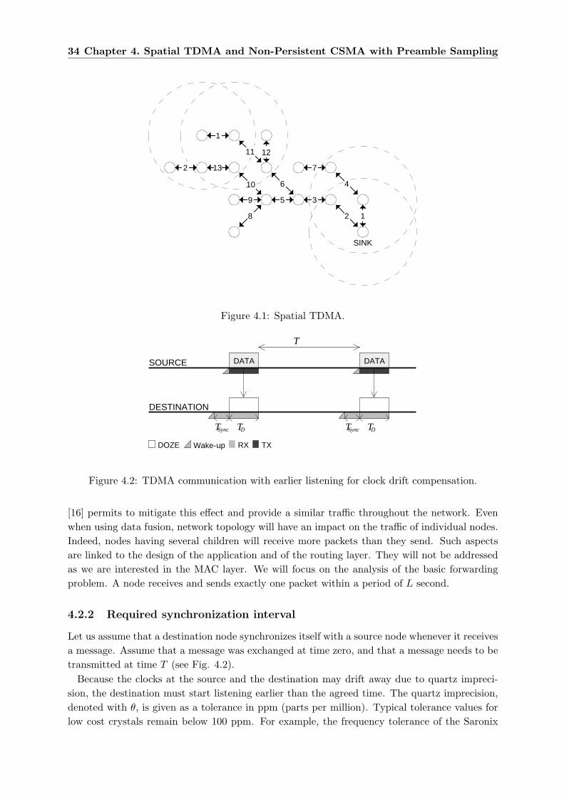
34 Chapter 4. Spatial TDMA and Non-Persistent CSMA with Preamble Sampling
11
6
2
3
7
1
4
5
10
13
12
9
1
2
SINK
8
Figure 4.1: Spatial TDMA.
SOURCE
DESTINATION
DATA
DOZE RX TX
T
TDTSync
Wake-up
DATA
TDTSync
Figure 4.2: TDMA communication with earlier listening for clock drift compensation.
[16] permits to mitigate this effect and provide a similar traffic throughout the network. Evenwhen using data fusion, network topology will have an impact on the traffic of individual nodes.Indeed, nodes having several children will receive more packets than they send. Such aspectsare linked to the design of the application and of the routing layer. They will not be addressedas we are interested in the MAC layer. We will focus on the analysis of the basic forwardingproblem. A node receives and sends exactly one packet within a period of L second.
4.2.2 Required synchronization interval
Let us assume that a destination node synchronizes itself with a source node whenever it receivesa message. Assume that a message was exchanged at time zero, and that a message needs to betransmitted at time T (see Fig. 4.2).
Because the clocks at the source and the destination may drift away due to quartz impreci-sion, the destination must start listening earlier than the agreed time. The quartz imprecision,denoted with θ, is given as a tolerance in ppm (parts per million). Typical tolerance values forlow cost crystals remain below 100 ppm. For example, the frequency tolerance of the Saronix
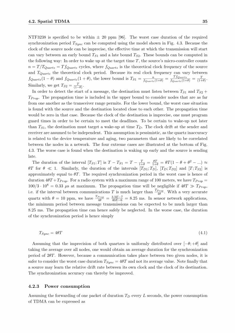
4.2. Spatial TDMA 35
NTF3238 is specified to be within ± 20 ppm [96]. The worst case duration of the requiredsynchronization period TSync can be computed using the model shown in Fig. 4.3. Because theclock of the source node can be imprecise, the effective time at which the transmission will startcan vary between an early bound TS1 and a late bound TS2. These bounds can be computed inthe following way: In order to wake up at the target time T , the source’s micro-controller countsn = T/TQuartz = TfQuartz cycles, where fQuartz is the theoretical clock frequency of the sourceand TQuartz the theoretical clock period. Because its real clock frequency can vary betweenfQuartz(1 − θ) and fQuartz(1 + θ), the lower bound is TS1 = n
fQuartz(1+θ) = TfQuartz
fQuartz(1+θ) = T(1+θ) .
Similarly, we get TS2 = T(1−θ) .
In order to detect the start of a message, the destination must listen between TS1 and TS2 +TProp. The propagation time is included in the upper bound to consider nodes that are as farfrom one another as the transceiver range permits. For the lower bound, the worst case situationis found with the source and the destination located close to each other. The propagation timewould be zero in that case. Because the clock of the destination is imprecise, one must programguard times in order to be certain to meet the deadlines. To be certain to wake-up not laterthan TS1, the destination must target a wake-up at time TD. The clock drift at the sender andreceiver are assumed to be independent. This assumption is pessimistic, as the quartz inaccuracyis related to the device temperature and aging, two parameters that are likely to be correlatedbetween the nodes in a network. The four extreme cases are illustrated at the bottom of Fig.4.3. The worse case is found when the destination is waking up early and the source is sendinglate.
The duration of the interval [TS1; T ] is T − TS1 = T − T1+θ = θT
1+θ = θT (1 − θ + θ2 − ...) ≈θT for θ ¿ 1. Similarly, the duration of the intervals [TD1; TD], [TD; TD2] and [T ; TS2] isapproximately equal to θT . The required synchronization period in the worst case is hence ofduration 4θT +TProp. For a radio system with a maximum range of 100 meters, we have TProp =100/3 · 108 = 0.33 µs at maximum. The propagation time will be negligible if 4θT À TProp,i.e. if the interval between communications T is much larger than TProp
4θ . With a very accuratequartz with θ = 10 ppm, we have TProp
4θ = 3.3E−740E−6 = 8.25 ms. In sensor network applications,
the minimum period between message transmissions can be expected to be much larger than8.25 ms. The propagation time can hence safely be neglected. In the worse case, the durationof the synchronization period is hence simply
TSync = 4θT (4.1)
Assuming that the imprecision of both quartzes is uniformly distributed over [−θ; +θ] andtaking the average over all nodes, one would obtain an average duration for the synchronizationperiod of 2θT . However, because a communication takes place between two given nodes, it issafer to consider the worst case duration TSync = 4θT and not its average value. Note finally thata source may learn the relative drift rate between its own clock and the clock of its destination.The synchronization accuracy can thereby be improved.
4.2.3 Power consumption
Assuming the forwarding of one packet of duration TD every L seconds, the power consumptionof TDMA can be expressed as
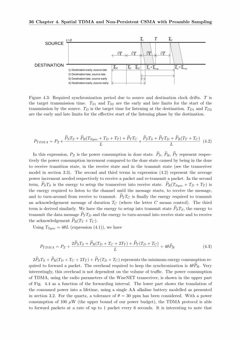
36 Chapter 4. Spatial TDMA and Non-Persistent CSMA with Preamble Sampling
S2SOURCE
DESTINATION
Tt=0
TProp+TProp+1) Destination early, source late
2) Destination late, source late
3) Destination late, source early
4) Destination early, source early
TS1 T
TS1 TS2
T T T T
TD1 TD TD2
Figure 4.3: Required synchronization period due to source and destination clock drifts. T isthe target transmission time. TS1 and TS2 are the early and late limits for the start of thetransmission by the source. TD is the target time for listening at the destination. TD1 and TD2
are the early and late limits for the effective start of the listening phase by the destination.
PTDMA = PZ +PSTS + PR(TSync + TD + TT ) + PT TC
L+
PSTS + PT TD + PR(TT + TC)L
(4.2)
In this expression, PZ is the power consumption in doze state. PS , PR, PT represent respec-tively the power consumption increment compared to the doze state caused by being in the dozeto receive transition state, in the receive state and in the transmit state (see the transceivermodel in section 3.3). The second and third terms in expression (4.2) represent the averagepower increment needed respectively to receive a packet and re-transmit a packet. In the secondterm, PSTS is the energy to setup the transceiver into receive state. PR(TSync + TD + TT ) isthe energy required to listen to the channel until the message starts, to receive the message,and to turn-around from receive to transmit. PT TC is finally the energy required to transmitan acknowledgement message of duration TC (where the letter C means control). The thirdterm is derived similarly. We have the energy to setup into transmit state PSTS , the energy totransmit the data message PT TD and the energy to turn-around into receive state and to receivethe acknowledgement PR(TT + TC).
Using TSync = 4θL (expression (4.1)), we have
PTDMA = PZ +2PSTS + PR(TD + TC + 2TT ) + PT (TD + TC)
L+ 4θPR (4.3)
2PSTS + PR(TD + TC + 2TT ) + PT (TD + TC) represents the minimum energy consumption re-quired to forward a packet. The overhead required to keep the synchronization is 4θPR. Veryinterestingly, this overhead is not dependent on the volume of traffic. The power consumptionof TDMA, using the radio parameters of the WiseNET transceiver, is shown in the upper partof Fig. 4.4 as a function of the forwarding interval. The lower part shows the translation ofthe consumed power into a lifetime, using a single AA alkaline battery modelled as presentedin section 3.2. For the quartz, a tolerance of θ = 30 ppm has been considered. With a powerconsumption of 100 µW (the upper bound of our power budget), the TDMA protocol is ableto forward packets at a rate of up to 1 packet every 6 seconds. It is interesting to note that
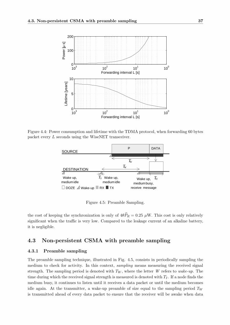
4.3. Non-persistent CSMA with preamble sampling 37
100
101
102
103
0
100
200
Forwarding interval L [s]
Pow
er [µ
s]
100
101
102
103
0
5
10
Forwarding interval L [s]
Life
time
[yea
rs]
Figure 4.4: Power consumption and lifetime with the TDMA protocol, when forwarding 60 bytespacket every L seconds using the WiseNET transceiver.
SOURCE
DESTINATION
P DATA
Wake up,mediumidle
Wake up,mediumidle
Wake up, mediumbusy,
receive messageDOZE RX TX
TW
TD
TW
TS
Wake-up
Figure 4.5: Preamble Sampling.
the cost of keeping the synchronization is only of 4θPR = 0.25 µW. This cost is only relativelysignificant when the traffic is very low. Compared to the leakage current of an alkaline battery,it is negligible.
4.3 Non-persistent CSMA with preamble sampling
4.3.1 Preamble sampling
The preamble sampling technique, illustrated in Fig. 4.5, consists in periodically sampling themedium to check for activity. In this context, sampling means measuring the received signalstrength. The sampling period is denoted with TW , where the letter W refers to wake-up. Thetime during which the received signal strength is measured is denoted with TI . If a node finds themedium busy, it continues to listen until it receives a data packet or until the medium becomesidle again. At the transmitter, a wake-up preamble of size equal to the sampling period TW
is transmitted ahead of every data packet to ensure that the receiver will be awake when data
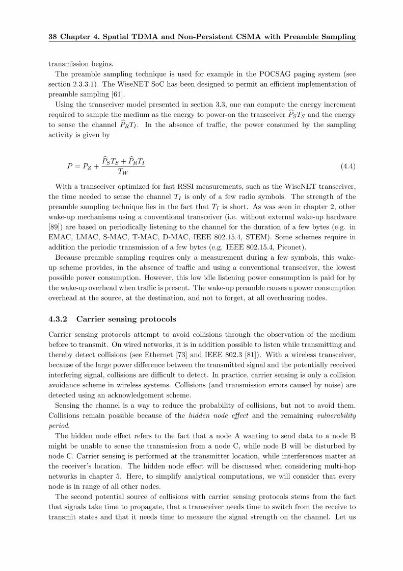
38 Chapter 4. Spatial TDMA and Non-Persistent CSMA with Preamble Sampling
transmission begins.The preamble sampling technique is used for example in the POCSAG paging system (see
section 2.3.3.1). The WiseNET SoC has been designed to permit an efficient implementation ofpreamble sampling [61].
Using the transceiver model presented in section 3.3, one can compute the energy incrementrequired to sample the medium as the energy to power-on the transceiver PSTS and the energyto sense the channel PRTI . In the absence of traffic, the power consumed by the samplingactivity is given by
P = PZ +PSTS + PRTI
TW(4.4)
With a transceiver optimized for fast RSSI measurements, such as the WiseNET transceiver,the time needed to sense the channel TI is only of a few radio symbols. The strength of thepreamble sampling technique lies in the fact that TI is short. As was seen in chapter 2, otherwake-up mechanisms using a conventional transceiver (i.e. without external wake-up hardware[89]) are based on periodically listening to the channel for the duration of a few bytes (e.g. inEMAC, LMAC, S-MAC, T-MAC, D-MAC, IEEE 802.15.4, STEM). Some schemes require inaddition the periodic transmission of a few bytes (e.g. IEEE 802.15.4, Piconet).
Because preamble sampling requires only a measurement during a few symbols, this wake-up scheme provides, in the absence of traffic and using a conventional transceiver, the lowestpossible power consumption. However, this low idle listening power consumption is paid for bythe wake-up overhead when traffic is present. The wake-up preamble causes a power consumptionoverhead at the source, at the destination, and not to forget, at all overhearing nodes.
4.3.2 Carrier sensing protocols
Carrier sensing protocols attempt to avoid collisions through the observation of the mediumbefore to transmit. On wired networks, it is in addition possible to listen while transmitting andthereby detect collisions (see Ethernet [73] and IEEE 802.3 [81]). With a wireless transceiver,because of the large power difference between the transmitted signal and the potentially receivedinterfering signal, collisions are difficult to detect. In practice, carrier sensing is only a collisionavoidance scheme in wireless systems. Collisions (and transmission errors caused by noise) aredetected using an acknowledgement scheme.
Sensing the channel is a way to reduce the probability of collisions, but not to avoid them.Collisions remain possible because of the hidden node effect and the remaining vulnerabilityperiod.
The hidden node effect refers to the fact that a node A wanting to send data to a node Bmight be unable to sense the transmission from a node C, while node B will be disturbed bynode C. Carrier sensing is performed at the transmitter location, while interferences matter atthe receiver’s location. The hidden node effect will be discussed when considering multi-hopnetworks in chapter 5. Here, to simplify analytical computations, we will consider that everynode is in range of all other nodes.
The second potential source of collisions with carrier sensing protocols stems from the factthat signals take time to propagate, that a transceiver needs time to switch from the receive totransmit states and that it needs time to measure the signal strength on the channel. Let us
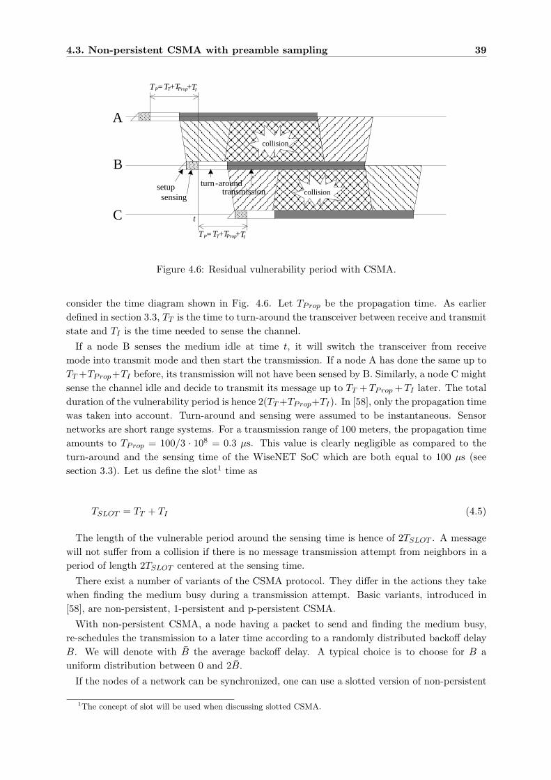
4.3. Non-persistent CSMA with preamble sampling 39
A
B
C
sensing
turn-aroundsetup transmission collision
collision
t
TT TI+TProp+T =P
TT TI+TProp+T =P
Figure 4.6: Residual vulnerability period with CSMA.
consider the time diagram shown in Fig. 4.6. Let TProp be the propagation time. As earlierdefined in section 3.3, TT is the time to turn-around the transceiver between receive and transmitstate and TI is the time needed to sense the channel.
If a node B senses the medium idle at time t, it will switch the transceiver from receivemode into transmit mode and then start the transmission. If a node A has done the same up toTT +TProp+TI before, its transmission will not have been sensed by B. Similarly, a node C mightsense the channel idle and decide to transmit its message up to TT +TProp +TI later. The totalduration of the vulnerability period is hence 2(TT +TProp+TI). In [58], only the propagation timewas taken into account. Turn-around and sensing were assumed to be instantaneous. Sensornetworks are short range systems. For a transmission range of 100 meters, the propagation timeamounts to TProp = 100/3 · 108 = 0.3 µs. This value is clearly negligible as compared to theturn-around and the sensing time of the WiseNET SoC which are both equal to 100 µs (seesection 3.3). Let us define the slot1 time as
TSLOT = TT + TI (4.5)
The length of the vulnerable period around the sensing time is hence of 2TSLOT . A messagewill not suffer from a collision if there is no message transmission attempt from neighbors in aperiod of length 2TSLOT centered at the sensing time.
There exist a number of variants of the CSMA protocol. They differ in the actions they takewhen finding the medium busy during a transmission attempt. Basic variants, introduced in[58], are non-persistent, 1-persistent and p-persistent CSMA.
With non-persistent CSMA, a node having a packet to send and finding the medium busy,re-schedules the transmission to a later time according to a randomly distributed backoff delayB. We will denote with B the average backoff delay. A typical choice is to choose for B auniform distribution between 0 and 2B.
If the nodes of a network can be synchronized, one can use a slotted version of non-persistent
1The concept of slot will be used when discussing slotted CSMA.
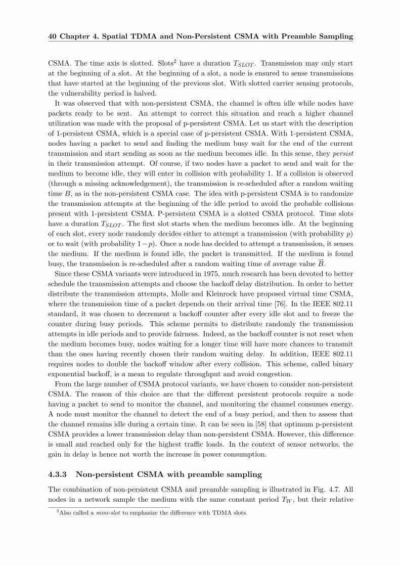
40 Chapter 4. Spatial TDMA and Non-Persistent CSMA with Preamble Sampling
CSMA. The time axis is slotted. Slots2 have a duration TSLOT . Transmission may only startat the beginning of a slot. At the beginning of a slot, a node is ensured to sense transmissionsthat have started at the beginning of the previous slot. With slotted carrier sensing protocols,the vulnerability period is halved.
It was observed that with non-persistent CSMA, the channel is often idle while nodes havepackets ready to be sent. An attempt to correct this situation and reach a higher channelutilization was made with the proposal of p-persistent CSMA. Let us start with the descriptionof 1-persistent CSMA, which is a special case of p-persistent CSMA. With 1-persistent CSMA,nodes having a packet to send and finding the medium busy wait for the end of the currenttransmission and start sending as soon as the medium becomes idle. In this sense, they persistin their transmission attempt. Of course, if two nodes have a packet to send and wait for themedium to become idle, they will enter in collision with probability 1. If a collision is observed(through a missing acknowledgement), the transmission is re-scheduled after a random waitingtime B, as in the non-persistent CSMA case. The idea with p-persistent CSMA is to randomizethe transmission attempts at the beginning of the idle period to avoid the probable collisionspresent with 1-persistent CSMA. P-persistent CSMA is a slotted CSMA protocol. Time slotshave a duration TSLOT . The first slot starts when the medium becomes idle. At the beginningof each slot, every node randomly decides either to attempt a transmission (with probability p)or to wait (with probability 1−p). Once a node has decided to attempt a transmission, it sensesthe medium. If the medium is found idle, the packet is transmitted. If the medium is foundbusy, the transmission is re-scheduled after a random waiting time of average value B.
Since these CSMA variants were introduced in 1975, much research has been devoted to betterschedule the transmission attempts and choose the backoff delay distribution. In order to betterdistribute the transmission attempts, Molle and Kleinrock have proposed virtual time CSMA,where the transmission time of a packet depends on their arrival time [76]. In the IEEE 802.11standard, it was chosen to decrement a backoff counter after every idle slot and to freeze thecounter during busy periods. This scheme permits to distribute randomly the transmissionattempts in idle periods and to provide fairness. Indeed, as the backoff counter is not reset whenthe medium becomes busy, nodes waiting for a longer time will have more chances to transmitthan the ones having recently chosen their random waiting delay. In addition, IEEE 802.11requires nodes to double the backoff window after every collision. This scheme, called binaryexponential backoff, is a mean to regulate throughput and avoid congestion.
From the large number of CSMA protocol variants, we have chosen to consider non-persistentCSMA. The reason of this choice are that the different persistent protocols require a nodehaving a packet to send to monitor the channel, and monitoring the channel consumes energy.A node must monitor the channel to detect the end of a busy period, and then to assess thatthe channel remains idle during a certain time. It can be seen in [58] that optimum p-persistentCSMA provides a lower transmission delay than non-persistent CSMA. However, this differenceis small and reached only for the highest traffic loads. In the context of sensor networks, thegain in delay is hence not worth the increase in power consumption.
4.3.3 Non-persistent CSMA with preamble sampling
The combination of non-persistent CSMA and preamble sampling is illustrated in Fig. 4.7. Allnodes in a network sample the medium with the same constant period TW , but their relative
2Also called a mini-slot to emphasize the difference with TDMA slots.
4.3. Non-persistent CSMA with preamble sampling 41
SOURCE
DESTINATIONA
P DATA
Wake up,mediumidle
Wake up,mediumidle
Wake up, mediumbusy,
receive messageDOZE RX TX
TW
TD TT TC
TW
Wake-up
Arrival,transmit if mediumidle,
defer if mediumbusy
Figure 4.7: Non-persistent CSMA with preamble sampling.
1
2
N
MAC
MAC
MAC
CHANNELS
g
g
g
transmission attempts (carrier sensing)feedback: channel busy or missing ack
Figure 4.8: System model for NP-CSMA analysis.
sampling schedule offsets are independent. A node having a packet to send will precede it witha preamble of length TW . Before transmitting, a node senses the medium. If the medium isbusy, the radio is turned off and the transmission attempt is deferred after a randomly chosenwaiting delay of average value B.
If, during a transmission attempt, a node finds the medium busy, one could be tempted tokeep the radio in receive mode to attempt to receive a message. In order to save energy, it isbetter to turn the transceiver off, and wait for the next scheduled periodic wake-up time, whichwill be soon enough to catch any transmission.
The performance analysis of NP-CSMA-PS is based on the renewal theory described by Klein-rock and Tobagi in [58]. Their method has been adapted for the analysis of the preamble sam-pling technique and extended to derive power consumption information. We assume a networkof N nodes, where every node is in range of every other node. Poisson traffic with rate λ isgenerated by every node and addressed to any other node. The sum of the initial transmissionattempts and the re-transmission attempts is assumed to be distributed according to a Poissonprocess of rate g. It is important to note that g is the attempt rate and not the rate with whichpackets are transmitted. The global attempt rate considering all nodes is Ng. The amountof traffic transmitted with success is measured with the throughput S ∈ [0; 1]. As long as thesystem remains stable, we have S = Nλ/TD. The system model is illustrated in Fig. 4.8.
4.3.3.1 Throughput
The average throughput can be computed considering the average duration of idle and busyperiods. An idle period starts at the end of the transmission of a packet and ends at the start
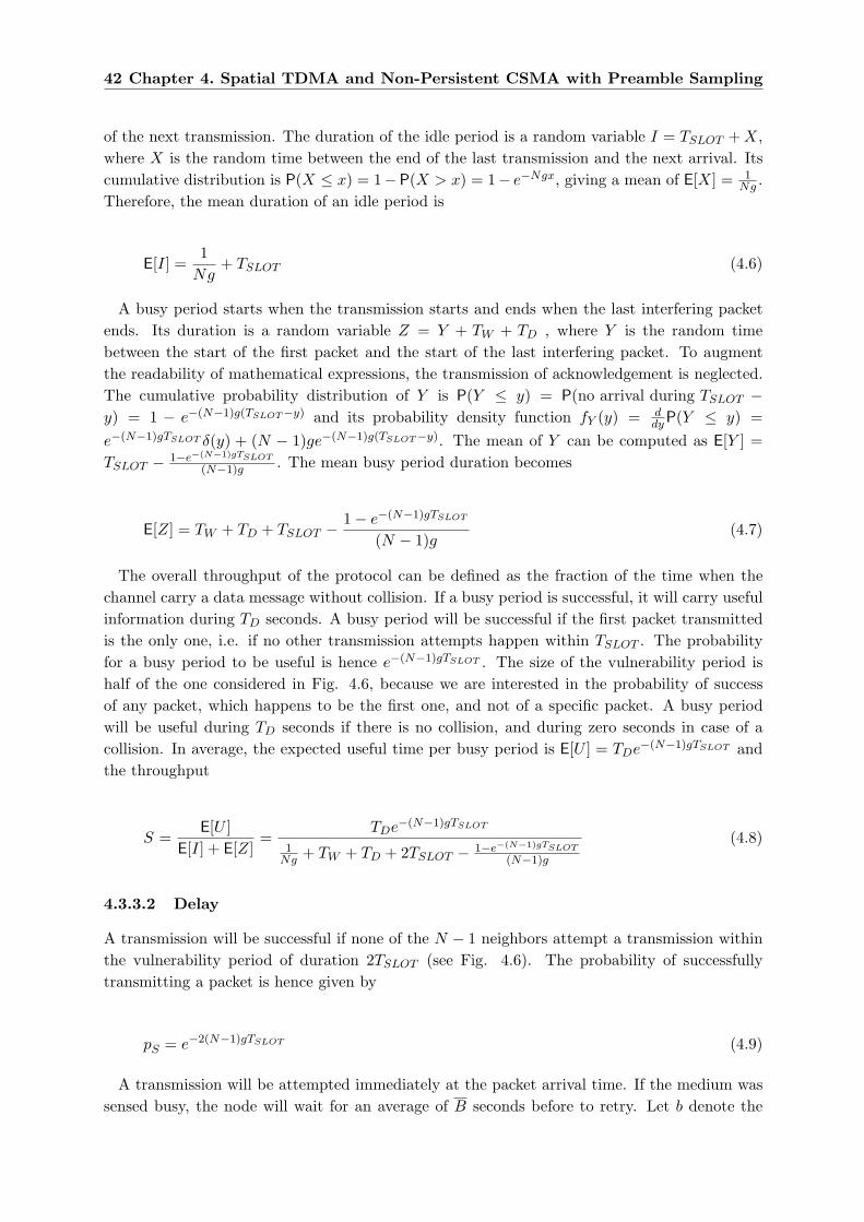
42 Chapter 4. Spatial TDMA and Non-Persistent CSMA with Preamble Sampling
of the next transmission. The duration of the idle period is a random variable I = TSLOT + X,where X is the random time between the end of the last transmission and the next arrival. Itscumulative distribution is P(X ≤ x) = 1−P(X > x) = 1− e−Ngx, giving a mean of E[X] = 1
Ng .Therefore, the mean duration of an idle period is
E[I] =1
Ng+ TSLOT (4.6)
A busy period starts when the transmission starts and ends when the last interfering packetends. Its duration is a random variable Z = Y + TW + TD , where Y is the random timebetween the start of the first packet and the start of the last interfering packet. To augmentthe readability of mathematical expressions, the transmission of acknowledgement is neglected.The cumulative probability distribution of Y is P(Y ≤ y) = P(no arrival during TSLOT −y) = 1 − e−(N−1)g(TSLOT−y) and its probability density function fY (y) = d
dyP(Y ≤ y) =e−(N−1)gTSLOT δ(y) + (N − 1)ge−(N−1)g(TSLOT−y). The mean of Y can be computed as E[Y ] =TSLOT − 1−e−(N−1)gTSLOT
(N−1)g . The mean busy period duration becomes
E[Z] = TW + TD + TSLOT − 1− e−(N−1)gTSLOT
(N − 1)g(4.7)
The overall throughput of the protocol can be defined as the fraction of the time when thechannel carry a data message without collision. If a busy period is successful, it will carry usefulinformation during TD seconds. A busy period will be successful if the first packet transmittedis the only one, i.e. if no other transmission attempts happen within TSLOT . The probabilityfor a busy period to be useful is hence e−(N−1)gTSLOT . The size of the vulnerability period ishalf of the one considered in Fig. 4.6, because we are interested in the probability of successof any packet, which happens to be the first one, and not of a specific packet. A busy periodwill be useful during TD seconds if there is no collision, and during zero seconds in case of acollision. In average, the expected useful time per busy period is E[U ] = TDe−(N−1)gTSLOT andthe throughput
S =E[U ]
E[I] + E[Z]=
TDe−(N−1)gTSLOT
1Ng + TW + TD + 2TSLOT − 1−e−(N−1)gTSLOT
(N−1)g
(4.8)
4.3.3.2 Delay
A transmission will be successful if none of the N − 1 neighbors attempt a transmission withinthe vulnerability period of duration 2TSLOT (see Fig. 4.6). The probability of successfullytransmitting a packet is hence given by
pS = e−2(N−1)gTSLOT (4.9)
A transmission will be attempted immediately at the packet arrival time. If the medium wassensed busy, the node will wait for an average of B seconds before to retry. Let b denote the
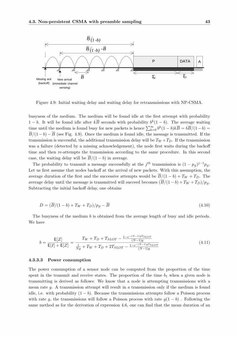
4.3. Non-persistent CSMA with preamble sampling 43
P DATA
TW TDB
B (1 -b)
New arrival(immediate channel
sensing)
Missing ack(backoff)
B (1 -b)
-B
A
Figure 4.9: Initial waiting delay and waiting delay for retransmissions with NP-CSMA.
busyness of the medium. The medium will be found idle at the first attempt with probability1 − b. It will be found idle after kB seconds with probability bk(1 − b). The average waitingtime until the medium is found busy for new packets is hence
∑∞k=0 bk(1− b)kB = bB/(1− b) =
B/(1− b)−B (see Fig. 4.9). Once the medium is found idle, the message is transmitted. If thetransmission is successful, the additional transmission delay will be TW +TD. If the transmissionwas a failure (detected by a missing acknowledgement), the node first waits during the backofftime and then re-attempts the transmission according to the same procedure. In this secondcase, the waiting delay will be B/(1− b) in average.
The probability to transmit a message successfully at the jth transmission is (1 − pS)j−1pS .Let us first assume that nodes backoff at the arrival of new packets. With this assumption, theaverage duration of the first and the successive attempts would be B/(1 − b) + TW + TD. Theaverage delay until the message is transmitted will succeed becomes (B/(1− b) + TW + TD)/pS .Subtracting the initial backoff delay, one obtains
D = (B/(1− b) + TW + TD)/pS −B (4.10)
The busyness of the medium b is obtained from the average length of busy and idle periods.We have
b =E[Z]
E[I] + E[Z]=
TW + TD + TSLOT − 1−e−(N−1)gTSLOT
(N−1)g
1Ng + TW + TD + 2TSLOT − 1−e−(N−1)gTSLOT
(N−1)g
(4.11)
4.3.3.3 Power consumption
The power consumption of a sensor node can be computed from the proportion of the timespent in the transmit and receive states. The proportion of the time b1 when a given node istransmitting is derived as follows: We know that a node is attempting transmissions with amean rate g. A transmission attempt will result in a transmission only if the medium is foundidle, i.e. with probability (1− b). Because the transmissions attempts follow a Poisson processwith rate g, the transmissions will follow a Poisson process with rate g(1 − b) . Following thesame method as for the derivation of expression 4.6, one can find that the mean duration of an
44 Chapter 4. Spatial TDMA and Non-Persistent CSMA with Preamble Sampling
idle period at the transmitter is given by
E[I1] =1
(1− b)g+ TSLOT (4.12)
The mean duration of a busy period at the transmitter being simply the length of a messageE[Z1] = TW + TD, we obtain
b1 =E[Z1]
E[I1] + E[Z1]=
TW + TD1
(1−b)g + TSLOT + TW + TD(4.13)
A sensor node periodically samples the medium. If the medium is found busy, it will listenuntil a message is received. The medium will be busy with transmission from others with aprobability (b− b1). If the medium was found busy, a node will listen to the transmission untilthe data part is received. In average, the listening duration will be approximately equal toTW /2 (here we assume that TW À TD). As a node samples the medium every TW seconds,the proportion of the time spent listening is hence given by (b− b1)/2. Using the elementsintroduced, one can express the mean consumed power as
P = PZ +PSTS + PRTI
TW+ b1PT +
(b − b1)2
PR (4.14)
4.3.4 Regular and genie aided NP-CSMA
We will compare the performances of NP-CSMA-PS with those of the regular and genie aidedNP-CSMA protocols. The performance parameters of the regular NP-CSMA protocol can beobtained by setting TW = 0 in equations 4.8, 4.10, 4.11, 4.13 and 4.14. We have
SC =TDe−(N−1)gTSLOT
1Ng + TD + 2TSLOT − 1−e−(N−1)gTSLOT
(N−1)g
(4.15)
bC =TD + TSLOT − 1−e−(N−1)gTSLOT
Ng
1Ng + TD + 2TSLOT − 1−e−(N−1)gTSLOT
(N−1)g
(4.16)
bC1 =
TD1
(1−bC)g+ TSLOT + TD
(4.17)
DC =TD + B
(1− bC)pCS
−B (4.18)
With regular CSMA, a node is either in transmit or in receive state. The mean power con-sumption is hence
4.3. Non-persistent CSMA with preamble sampling 45
PC = PZ + bC1 PT + (1− bC
1 )PR (4.19)
The preamble sampling technique is a mean to mitigate idle listening. In order to measure theperformance of preamble sampling against an absolute benchmark, we introduce the concept ofgenie aided non-persistent CSMA. In this protocol, as genie tells to each node when the channelis busy. The genie informs the nodes TS seconds in advance such that they have enough time topower on their radio. A node hence doesn’t spend any time listening to an idle channel. Thisconcept helps measuring what could be hopefully approached by feasible methods attemptingto replace the genie. Note that this protocol, although helped by a genie, is not yet ideal. Itremoves the idle listening overhead, but not the overhearing overhead and the collisions.
The mean power consumed by a node using GA-NP-CSMA is the power consumed for recep-tion when the channel is busy because of the transmissions from the neighbors, plus the powerconsumed when transmitting itself. We have
PGC = PZ + bC1 PT + (bC − bC
1 )PR (4.20)
The other performance characteristics remain unchanged from NP-CSMA.
4.3.5 Performance evaluation
Fig. 4.10 shows the performance of NP-CSMA-PS as a function of the global attempt rate andfor three different values of the sampling period (50, 200 and 500 ms). The three first plots showthe throughput, the delay and the power consumption. The fourth plot shows the lifetime thatcan be reached with one AA alkaline battery using the model presented in section 3.2.
It can be observed that the mean power consumption of the regular NP-CSMA protocolcannot decrease below 2.1 mW, the power consumption in receive mode. NP-CSMA-PS canreach a power consumption below 100 µW when the traffic is low. A comparison with GA-NP-CSMA shows the power consumption overhead introduced by preamble sampling. In high trafficconditions, the power consumption of GA-NP-CSMA becomes larger than the one of NP-CSMA-PS. This a-priori astonishing behavior is caused by the fact that, when using NP-CSMA-PS,a node goes back to sleep after having received a packet. It will wake-up only at the nextpredefined sampling instant, even if the medium becomes busy earlier. With GA-NP-CSMA, anode will wake up as soon as the medium because busy and hence consume more energy. Thisportion of the curves is anyway of little interest as most packets are lost due to buffer overflowwith all three protocols.
The power consumption is best compared when looking at the resulting lifetime in the bottomplot. It can be observed that different sizes for the wake-up preambles are optimum for differentamounts of transported traffic.
The throughput is shown in bits per second units, obtained by multiplying S with 25000,the bit rate. This plot shows that the wake-up preambles cause an important reduction inthe maximum throughput. In the low traffic region, it can be observed that the throughputgrows linearly with the attempt rate. In this region, every transmission attempt result in atransmission, and every transmission is successful.
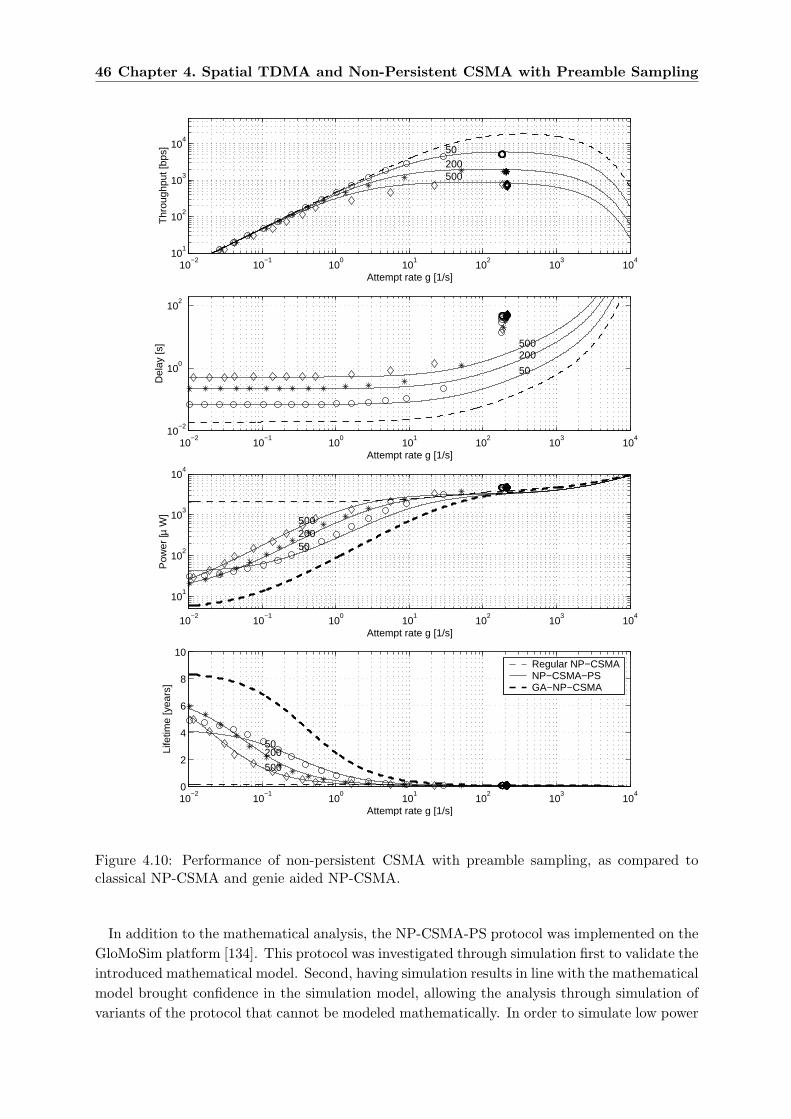
46 Chapter 4. Spatial TDMA and Non-Persistent CSMA with Preamble Sampling
10−2
10−1
100
101
102
103
104
101
102
103
104
50
Attempt rate g [1/s]
Thr
ough
put [
bps]
200500
10−2
10−1
100
101
102
103
104
10−2
100
102
50
Attempt rate g [1/s]
Del
ay [s
]
200500
10−2
10−1
100
101
102
103
104
101
102
103
104
50
Attempt rate g [1/s]
Pow
er [µ
W]
200500
10−2
10−1
100
101
102
103
104
0
2
4
6
8
10
50
Attempt rate g [1/s]
Life
time
[yea
rs]
200
500
Regular NP−CSMANP−CSMA−PSGA−NP−CSMA
Figure 4.10: Performance of non-persistent CSMA with preamble sampling, as compared toclassical NP-CSMA and genie aided NP-CSMA.
In addition to the mathematical analysis, the NP-CSMA-PS protocol was implemented on theGloMoSim platform [134]. This protocol was investigated through simulation first to validate theintroduced mathematical model. Second, having simulation results in line with the mathematicalmodel brought confidence in the simulation model, allowing the analysis through simulation ofvariants of the protocol that cannot be modeled mathematically. In order to simulate low power
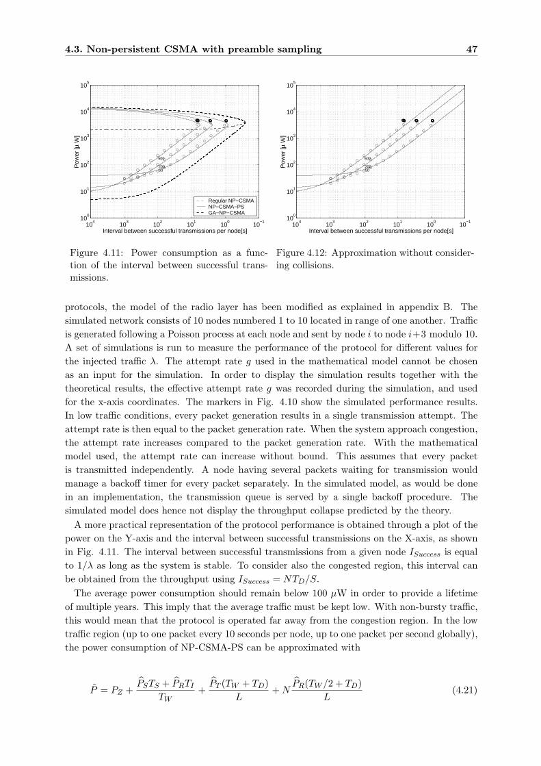
4.3. Non-persistent CSMA with preamble sampling 47
10−1
100
101
102
103
104
100
101
102
103
104
105
50200
500
Interval between successful transmissions per node[s]
Pow
er [µ
W]
Regular NP−CSMANP−CSMA−PSGA−NP−CSMA
Figure 4.11: Power consumption as a func-tion of the interval between successful trans-missions.
10−1
100
101
102
103
104
100
101
102
103
104
105
50200
500
Interval between successful transmissions per node[s]
Pow
er [µ
W]
Figure 4.12: Approximation without consider-ing collisions.
protocols, the model of the radio layer has been modified as explained in appendix B. Thesimulated network consists of 10 nodes numbered 1 to 10 located in range of one another. Trafficis generated following a Poisson process at each node and sent by node i to node i+3 modulo 10.A set of simulations is run to measure the performance of the protocol for different values forthe injected traffic λ. The attempt rate g used in the mathematical model cannot be chosenas an input for the simulation. In order to display the simulation results together with thetheoretical results, the effective attempt rate g was recorded during the simulation, and usedfor the x-axis coordinates. The markers in Fig. 4.10 show the simulated performance results.In low traffic conditions, every packet generation results in a single transmission attempt. Theattempt rate is then equal to the packet generation rate. When the system approach congestion,the attempt rate increases compared to the packet generation rate. With the mathematicalmodel used, the attempt rate can increase without bound. This assumes that every packetis transmitted independently. A node having several packets waiting for transmission wouldmanage a backoff timer for every packet separately. In the simulated model, as would be donein an implementation, the transmission queue is served by a single backoff procedure. Thesimulated model does hence not display the throughput collapse predicted by the theory.
A more practical representation of the protocol performance is obtained through a plot of thepower on the Y-axis and the interval between successful transmissions on the X-axis, as shownin Fig. 4.11. The interval between successful transmissions from a given node ISuccess is equalto 1/λ as long as the system is stable. To consider also the congested region, this interval canbe obtained from the throughput using ISuccess = NTD/S.
The average power consumption should remain below 100 µW in order to provide a lifetimeof multiple years. This imply that the average traffic must be kept low. With non-bursty traffic,this would mean that the protocol is operated far away from the congestion region. In the lowtraffic region (up to one packet every 10 seconds per node, up to one packet per second globally),the power consumption of NP-CSMA-PS can be approximated with
P = PZ +PSTS + PRTI
TW+
PT (TW + TD)L
+ NPR(TW /2 + TD)
L(4.21)
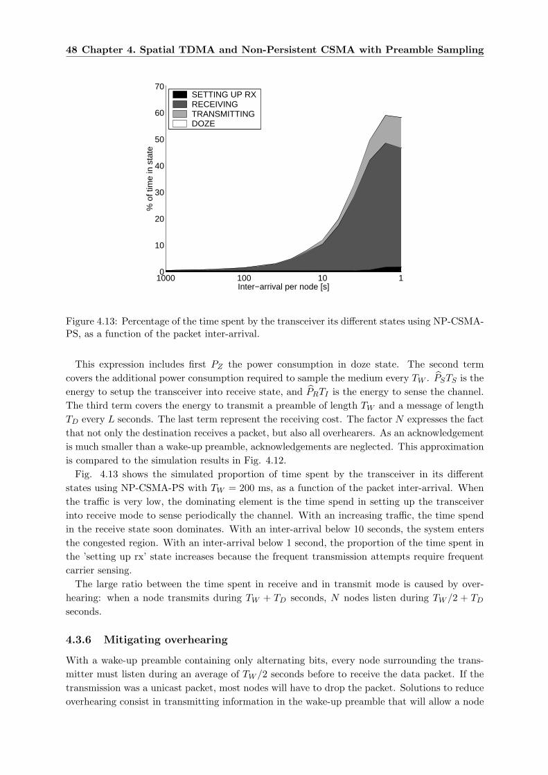
48 Chapter 4. Spatial TDMA and Non-Persistent CSMA with Preamble Sampling
11010010000
10
20
30
40
50
60
70
Inter−arrival per node [s]
% o
f tim
e in
sta
te
SETTING UP RXRECEIVINGTRANSMITTINGDOZE
Figure 4.13: Percentage of the time spent by the transceiver its different states using NP-CSMA-PS, as a function of the packet inter-arrival.
This expression includes first PZ the power consumption in doze state. The second termcovers the additional power consumption required to sample the medium every TW . PSTS is theenergy to setup the transceiver into receive state, and PRTI is the energy to sense the channel.The third term covers the energy to transmit a preamble of length TW and a message of lengthTD every L seconds. The last term represent the receiving cost. The factor N expresses the factthat not only the destination receives a packet, but also all overhearers. As an acknowledgementis much smaller than a wake-up preamble, acknowledgements are neglected. This approximationis compared to the simulation results in Fig. 4.12.
Fig. 4.13 shows the simulated proportion of time spent by the transceiver in its differentstates using NP-CSMA-PS with TW = 200 ms, as a function of the packet inter-arrival. Whenthe traffic is very low, the dominating element is the time spend in setting up the transceiverinto receive mode to sense periodically the channel. With an increasing traffic, the time spendin the receive state soon dominates. With an inter-arrival below 10 seconds, the system entersthe congested region. With an inter-arrival below 1 second, the proportion of the time spent inthe ’setting up rx’ state increases because the frequent transmission attempts require frequentcarrier sensing.
The large ratio between the time spent in receive and in transmit mode is caused by over-hearing: when a node transmits during TW + TD seconds, N nodes listen during TW /2 + TD
seconds.
4.3.6 Mitigating overhearing
With a wake-up preamble containing only alternating bits, every node surrounding the trans-mitter must listen during an average of TW /2 seconds before to receive the data packet. If thetransmission was a unicast packet, most nodes will have to drop the packet. Solutions to reduceoverhearing consist in transmitting information in the wake-up preamble that will allow a node
4.4. Comparing and combining S-TDMA and NP-CSMA-PS 49
to quickly know if it is the destination of the message. Such solutions include repeating anaddress information, or repeating the whole data message. The address information could bethe full length MAC address of the node. If the address is judged too long, one could transmita 8-bits hash of the address as proposed in the Hiperlan 1 standard [34].
The information present in the wake-up preamble can also be of use to the intended desti-nation of the transmission. If, together with the repeated address, a counter would indicatethe remaining length of the wake-up preamble, the destination could go back to sleep until thedata message is starting. If the whole message is repeated, a counter should indicate when theacknowledgement will have to be sent.
Repeating an address presents the advantage of allowing the overhearers to go back to sleepvery quickly. Repeating the whole message presents the advantage of adding redundancy. If thefirst copy of the message is not received correctly by the destination, it will have the possibilityto receive one of the following copies. Because of the forward error correction capability broughtby the repetition of the whole message in the wake-up preamble, we will consider this secondoption. Using this optimization, the power consumption of NP-CSMA-PS below the congestionregion becomes
P = PZ +PSTS + PRTI
TW+
PT (TW + TD)L
+ NPR(TD/2 + TD)
L(4.22)
The only difference between expressions (4.21) and (4.22) is that TW is replaced with TD inthe last term. The impact of this optimization is important when the node density N is largeand when the ratio between PT and PR is small.
4.4 Comparing and combining S-TDMA and NP-CSMA-PS
Fig. 4.14 shows the power consumption of S-TDMA (expression 4.3) and of NP-CSMA-PS withrepetition of the data message in the wake-up preamble (expression 4.22) as a function of thetransmission interval L. The power consumption of NP-CSMA-PS is drawn for three values ofthe wake-up period TW = 50, 200 and 500 ms. It can be observed that, for the transport ofperiodic traffic, S-TDMA is much more energy efficient that NP-CSMA-PS. It must however bekept in mind that this comparison is somehow unfair. We compare a protocol well suited for thetransport of periodic traffic and requiring network synchronization, with a protocol well suitedfor sporadic traffic and not requiring synchronization. The strength of NP-CSMA-PS is in beingable to provide a low power consumption when transporting sporadic traffic.
The work presented in this chapter lead us initially in the direction of using spatial TDMAfor the transport of frequent data traffic and NP-CSMA-PS for the transport of the supportingsignalling traffic. A transceiver capable of providing at least two frequency channels is required3.One channel is dedicated for the NP-CSMA-PS contention traffic and one channel is dedicatedfor the TDMA protocol. If the traffic is small, a single radio should be sufficient to bothcommunicate on the TDMA channel and periodically sample the medium on the NP-CSMA-PS channel. Using (4.3) and (4.22), the power consumption of the combined protocol can beapproximated with
3If more channels are available, a natural extension of Spatial TDMA would be Spatial Frequency and TimeDivision Multiple Access.
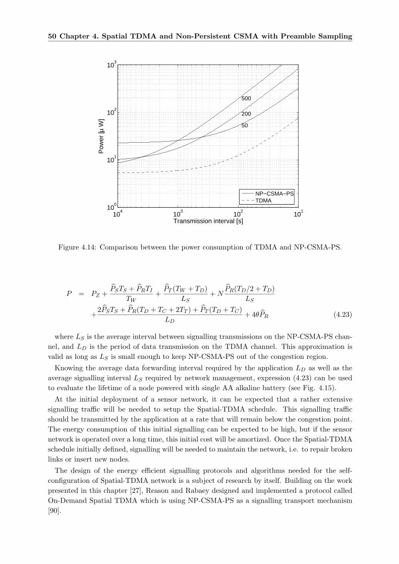
50 Chapter 4. Spatial TDMA and Non-Persistent CSMA with Preamble Sampling
101
102
103
104
100
101
102
103
50
200
500
Transmission interval [s]
Pow
er [µ
W]
NP−CSMA−PSTDMA
Figure 4.14: Comparison between the power consumption of TDMA and NP-CSMA-PS.
P = PZ +PSTS + PRTI
TW+
PT (TW + TD)LS
+ NPR(TD/2 + TD)
LS
+2PSTS + PR(TD + TC + 2TT ) + PT (TD + TC)
LD+ 4θPR (4.23)
where LS is the average interval between signalling transmissions on the NP-CSMA-PS chan-nel, and LD is the period of data transmission on the TDMA channel. This approximation isvalid as long as LS is small enough to keep NP-CSMA-PS out of the congestion region.
Knowing the average data forwarding interval required by the application LD as well as theaverage signalling interval LS required by network management, expression (4.23) can be usedto evaluate the lifetime of a node powered with single AA alkaline battery (see Fig. 4.15).
At the initial deployment of a sensor network, it can be expected that a rather extensivesignalling traffic will be needed to setup the Spatial-TDMA schedule. This signalling trafficshould be transmitted by the application at a rate that will remain below the congestion point.The energy consumption of this initial signalling can be expected to be high, but if the sensornetwork is operated over a long time, this initial cost will be amortized. Once the Spatial-TDMAschedule initially defined, signalling will be needed to maintain the network, i.e. to repair brokenlinks or insert new nodes.
The design of the energy efficient signalling protocols and algorithms needed for the self-configuration of Spatial-TDMA network is a subject of research by itself. Building on the workpresented in this chapter [27], Reason and Rabaey designed and implemented a protocol calledOn-Demand Spatial TDMA which is using NP-CSMA-PS as a signalling transport mechanism[90].
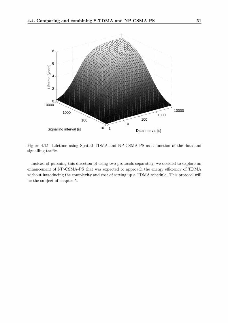
4.4. Comparing and combining S-TDMA and NP-CSMA-PS 51
110
1001000
10000
10
100
1000
100000
2
4
6
8
Data interval [s]Signalling interval [s]
Life
time
[yea
rs]
Figure 4.15: Lifetime using Spatial TDMA and NP-CSMA-PS as a function of the data andsignalling traffic.
Instead of pursuing this direction of using two protocols separately, we decided to explore anenhancement of NP-CSMA-PS that was expected to approach the energy efficiency of TDMAwithout introducing the complexity and cost of setting up a TDMA schedule. This protocol willbe the subject of chapter 5.

Chapter 5
WiseMAC for Multihop Wireless
Sensor Networks
5.1 Introduction
This chapter presents and analyzes a protocol that builds on NP-CSMA-PS to provide both alow average power consumption in low traffic conditions and a high energy efficiency in hightraffic conditions. This enhanced protocol has been called WiseMAC (Wireless sensor MAC)after the name of CSEM WiseNET project.
5.2 Protocol description
5.2.1 Overview
WiseMAC is a low power medium access control protocol designed for multi-hop wireless sensornetworks. As NP-CSMA-PS, presented in chapter 4, WiseMAC is a contention MAC protocoloperating on a single channel using non-persistent carrier sensing (NP-CSMA) for collisionavoidance. Idle listening is mitigated using the preamble sampling technique.
The drawback of NP-CSMA-PS is that the wake-up preamble represents a large overhead,leading to a poor energy efficiency. With WiseMAC, acknowledgements carry local synchroniza-tion information that is exploited to minimize the length of the wake-up preamble (see section5.2.2). Systematic collisions that would have been introduced through the synchronization aremitigated using a probabilistic medium reservation scheme (see section 5.2.3). Broadcast andunsynchronized unicast traffic use a random backoff procedure prior to transmission for colli-sion avoidance (see section 5.2.4). Overhearing is mitigated probabilistically when using a shortwake-up preamble and through the repetition of data frames within long wake-up preambles (seesection 5.2.5). Bursty traffic is transported energy efficiently thank to the ”more” bit, whichindicates when more packets are coming (see section 5.2.6). Interruption of data-ack dialoguesare avoided through the use of mandatory inter-frame spaces (see section 5.2.7). The receivethreshold is chosen well above the sensitivity to maximize useful wake-ups. The carrier sensingthreshold is chosen below the receive threshold to mitigate the hidden node effect (see section5.2.8). The tradeoffs made when choosing the sampling period are finally discussed in section5.2.9.
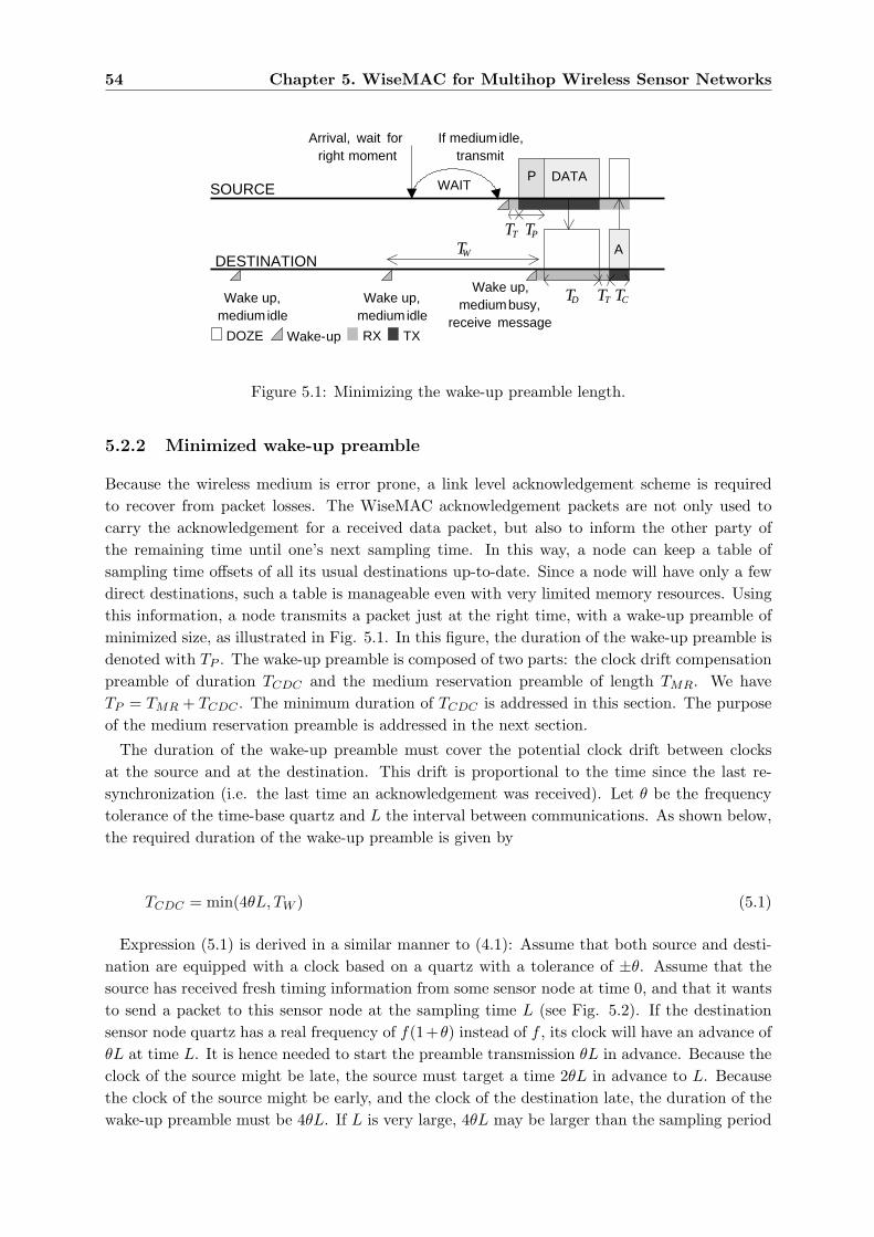
54 Chapter 5. WiseMAC for Multihop Wireless Sensor Networks
SOURCE
DESTINATIONA
WAIT
Arrival, wait forright moment
P DATA
If mediumidle,transmit
Wake up,mediumidle
Wake up,mediumidle
Wake up, mediumbusy,
receive message
TP
TW
DOZE RX TXWake-up
TD TCTT
TT
Figure 5.1: Minimizing the wake-up preamble length.
5.2.2 Minimized wake-up preamble
Because the wireless medium is error prone, a link level acknowledgement scheme is requiredto recover from packet losses. The WiseMAC acknowledgement packets are not only used tocarry the acknowledgement for a received data packet, but also to inform the other party ofthe remaining time until one’s next sampling time. In this way, a node can keep a table ofsampling time offsets of all its usual destinations up-to-date. Since a node will have only a fewdirect destinations, such a table is manageable even with very limited memory resources. Usingthis information, a node transmits a packet just at the right time, with a wake-up preamble ofminimized size, as illustrated in Fig. 5.1. In this figure, the duration of the wake-up preamble isdenoted with TP . The wake-up preamble is composed of two parts: the clock drift compensationpreamble of duration TCDC and the medium reservation preamble of length TMR. We haveTP = TMR + TCDC . The minimum duration of TCDC is addressed in this section. The purposeof the medium reservation preamble is addressed in the next section.
The duration of the wake-up preamble must cover the potential clock drift between clocksat the source and at the destination. This drift is proportional to the time since the last re-synchronization (i.e. the last time an acknowledgement was received). Let θ be the frequencytolerance of the time-base quartz and L the interval between communications. As shown below,the required duration of the wake-up preamble is given by
TCDC = min(4θL, TW ) (5.1)
Expression (5.1) is derived in a similar manner to (4.1): Assume that both source and desti-nation are equipped with a clock based on a quartz with a tolerance of ±θ. Assume that thesource has received fresh timing information from some sensor node at time 0, and that it wantsto send a packet to this sensor node at the sampling time L (see Fig. 5.2). If the destinationsensor node quartz has a real frequency of f(1+θ) instead of f , its clock will have an advance ofθL at time L. It is hence needed to start the preamble transmission θL in advance. Because theclock of the source might be late, the source must target a time 2θL in advance to L. Becausethe clock of the source might be early, and the clock of the destination late, the duration of thewake-up preamble must be 4θL. If L is very large, 4θL may be larger than the sampling period
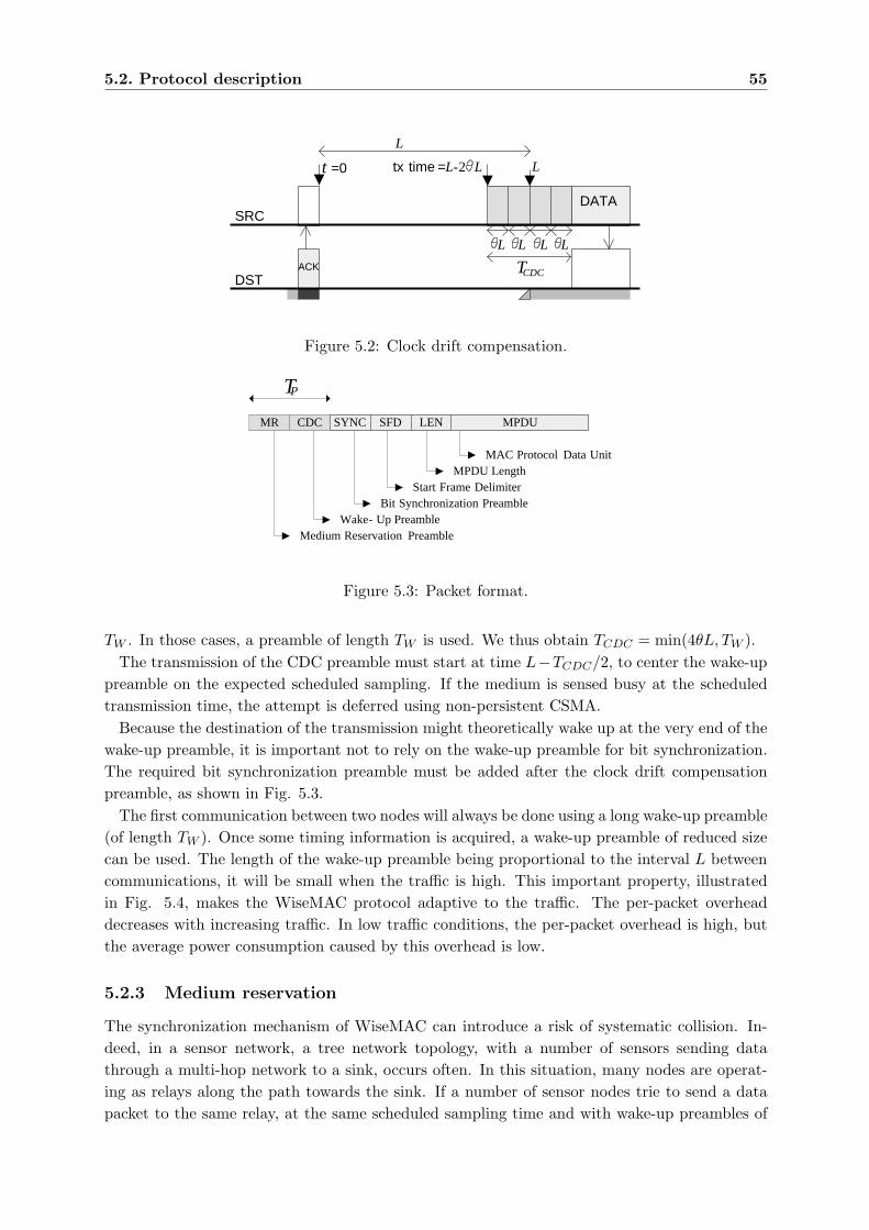
5.2. Protocol description 55
SRC
DST
t =0
DATA
ACK
tx time =L-2 L L
TCDC
L
L L L L
Figure 5.2: Clock drift compensation.
MAC Protocol Data Unit
Start Frame DelimiterBit Synchronization Preamble
Wake- Up PreambleMedium Reservation Preamble
SYNC SFD LEN MPDU
MPDU Length
TP
CDCMR
Figure 5.3: Packet format.
TW . In those cases, a preamble of length TW is used. We thus obtain TCDC = min(4θL, TW ).The transmission of the CDC preamble must start at time L−TCDC/2, to center the wake-up
preamble on the expected scheduled sampling. If the medium is sensed busy at the scheduledtransmission time, the attempt is deferred using non-persistent CSMA.
Because the destination of the transmission might theoretically wake up at the very end of thewake-up preamble, it is important not to rely on the wake-up preamble for bit synchronization.The required bit synchronization preamble must be added after the clock drift compensationpreamble, as shown in Fig. 5.3.
The first communication between two nodes will always be done using a long wake-up preamble(of length TW ). Once some timing information is acquired, a wake-up preamble of reduced sizecan be used. The length of the wake-up preamble being proportional to the interval L betweencommunications, it will be small when the traffic is high. This important property, illustratedin Fig. 5.4, makes the WiseMAC protocol adaptive to the traffic. The per-packet overheaddecreases with increasing traffic. In low traffic conditions, the per-packet overhead is high, butthe average power consumption caused by this overhead is low.
5.2.3 Medium reservation
The synchronization mechanism of WiseMAC can introduce a risk of systematic collision. In-deed, in a sensor network, a tree network topology, with a number of sensors sending datathrough a multi-hop network to a sink, occurs often. In this situation, many nodes are operat-ing as relays along the path towards the sink. If a number of sensor nodes trie to send a datapacket to the same relay, at the same scheduled sampling time and with wake-up preambles of
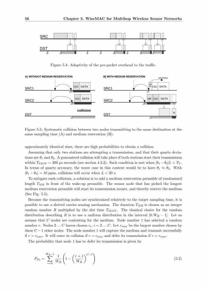
56 Chapter 5. WiseMAC for Multihop Wireless Sensor Networks
SRC
DST
Figure 5.4: Adaptivity of the per-packet overhead to the traffic.
SRC1CDC DATA
SRC2CDC DATA
DST
SRC1CDC DATA
SRC2CDC DATA
DST
MR
MR
A
DEFEREDA) WITHOUT MEDIUM RESERVATION B) WITH MEDIUM RESERVATION
collision
Figure 5.5: Systematic collision between two nodes transmitting to the same destination at thesame sampling time (A) and medium reservation (B).
approximately identical sizes, there are high probabilities to obtain a collision.Assuming that only two stations are attempting a transmission, and that their quartz devia-
tions are θ1 and θ2. A guaranteed collision will take place if both stations start their transmissionwithin TSLOT = 200 µs seconds (see section 4.3.2). Such condition is met when |θ1− θ2|L < TT .In terms of quartz accuracy, the worst case in this context would be to have θ1 ≈ θ2. With|θ1 − θ2| = 10 ppm, collisions will occur when L < 20 s.
To mitigate such collisions, a solution is to add a medium reservation preamble of randomizedlength TMR in front of the wake-up preamble. The sensor node that has picked the longestmedium reservation preamble will start its transmission sooner, and thereby reserve the medium(See Fig. 5.5).
Because the transmitting nodes are synchronized relatively to the target sampling time, it ispossible to use a slotted carrier sensing mechanism. The duration TMR is chosen as an integerrandom number R multiplied by the slot time TSLOT . The classical choice for the randomdistribution describing R is to use a uniform distribution in the interval [0;WR − 1]. Let usassume that C nodes are contenting for the medium. Node number 1 has selected a randomnumber r. Nodes 2 . . . C haven chosen ri, i = 2 . . . C. Let rmax be the largest number chosen bythese C−1 other nodes. The node number 1 will capture the medium and transmit successfullyif r > rmax. It will enter in collision if r = rmax and defer its transmission if r < rmax.
The probability that node 1 has to defer its transmission is given by
PD1 =WR−1∑
r=0
1WR
(1−
(r + 1WR
)C−1)
(5.2)
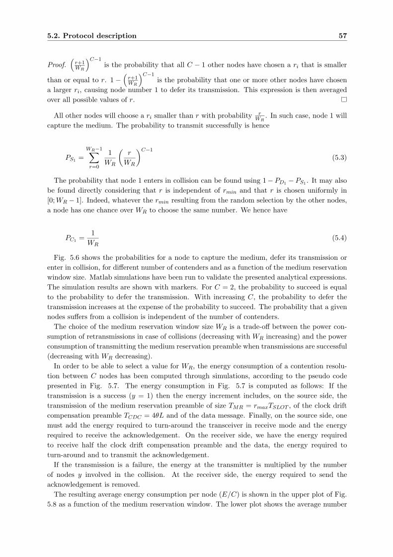
5.2. Protocol description 57
Proof.(
r+1WR
)C−1is the probability that all C − 1 other nodes have chosen a ri that is smaller
than or equal to r. 1 −(
r+1WR
)C−1is the probability that one or more other nodes have chosen
a larger ri, causing node number 1 to defer its transmission. This expression is then averagedover all possible values of r.
All other nodes will choose a ri smaller than r with probability rWR
. In such case, node 1 willcapture the medium. The probability to transmit successfully is hence
PS1 =WR−1∑
r=0
1WR
(r
WR
)C−1
(5.3)
The probability that node 1 enters in collision can be found using 1− PD1 − PS1 . It may alsobe found directly considering that r is independent of rmin and that r is chosen uniformly in[0;WR − 1]. Indeed, whatever the rmin resulting from the random selection by the other nodes,a node has one chance over WR to choose the same number. We hence have
PC1 =1
WR(5.4)
Fig. 5.6 shows the probabilities for a node to capture the medium, defer its transmission orenter in collision, for different number of contenders and as a function of the medium reservationwindow size. Matlab simulations have been run to validate the presented analytical expressions.The simulation results are shown with markers. For C = 2, the probability to succeed is equalto the probability to defer the transmission. With increasing C, the probability to defer thetransmission increases at the expense of the probability to succeed. The probability that a givennodes suffers from a collision is independent of the number of contenders.
The choice of the medium reservation window size WR is a trade-off between the power con-sumption of retransmissions in case of collisions (decreasing with WR increasing) and the powerconsumption of transmitting the medium reservation preamble when transmissions are successful(decreasing with WR decreasing).
In order to be able to select a value for WR, the energy consumption of a contention resolu-tion between C nodes has been computed through simulations, according to the pseudo codepresented in Fig. 5.7. The energy consumption in Fig. 5.7 is computed as follows: If thetransmission is a success (y = 1) then the energy increment includes, on the source side, thetransmission of the medium reservation preamble of size TMR = rmaxTSLOT , of the clock driftcompensation preamble TCDC = 4θL and of the data message. Finally, on the source side, onemust add the energy required to turn-around the transceiver in receive mode and the energyrequired to receive the acknowledgement. On the receiver side, we have the energy requiredto receive half the clock drift compensation preamble and the data, the energy required toturn-around and to transmit the acknowledgement.
If the transmission is a failure, the energy at the transmitter is multiplied by the numberof nodes y involved in the collision. At the receiver side, the energy required to send theacknowledgement is removed.
The resulting average energy consumption per node (E/C) is shown in the upper plot of Fig.5.8 as a function of the medium reservation window. The lower plot shows the average number
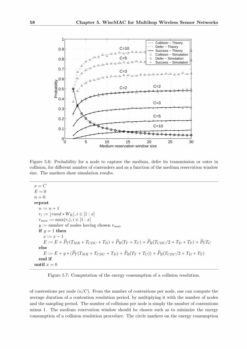
58 Chapter 5. WiseMAC for Multihop Wireless Sensor Networks
0 5 10 15 20 25 300
0.1
0.2
0.3
0.4
0.5
0.6
0.7
0.8
0.9
1
C=2 C=2
C=3
C=3
C=5
C=5
C=10
C=10
Medium reservation window size
Pro
babi
lity
Collision − TheoryDefer − TheorySuccess − TheoryCollision − SimulationDefer − SimulationSuccess − Simulation
Figure 5.6: Probability for a node to capture the medium, defer its transmission or enter incollision, for different number of contenders and as a function of the medium reservation windowsize. The markers show simulation results.
x = CE = 0n = 0repeat
n := n + 1ri := brand ∗WRc, i ∈ [1 : x]rmax := max(ri), i ∈ [1 : x]y := number of nodes having chosen rmax
if y = 1 thenx := x− 1E := E + PT (TMR + TCDC + TD) + PR(TT + TC) + PR(TCDC/2 + TD + TT ) + PT TC
elseE := E + y ∗ (PT (TMR + TCDC + TD) + PR(TT + TC)) + PR(TCDC/2 + TD + TT )
end ifuntil x = 0
Figure 5.7: Computation of the energy consumption of a collision resolution.
of contentions per node (n/C). From the number of contentions per node, one can compute theaverage duration of a contention resolution period, by multiplying it with the number of nodesand the sampling period. The number of collisions per node is simply the number of contentionsminus 1. The medium reservation window should be chosen such as to minimize the energyconsumption of a collision resolution procedure. The circle markers on the energy consumption
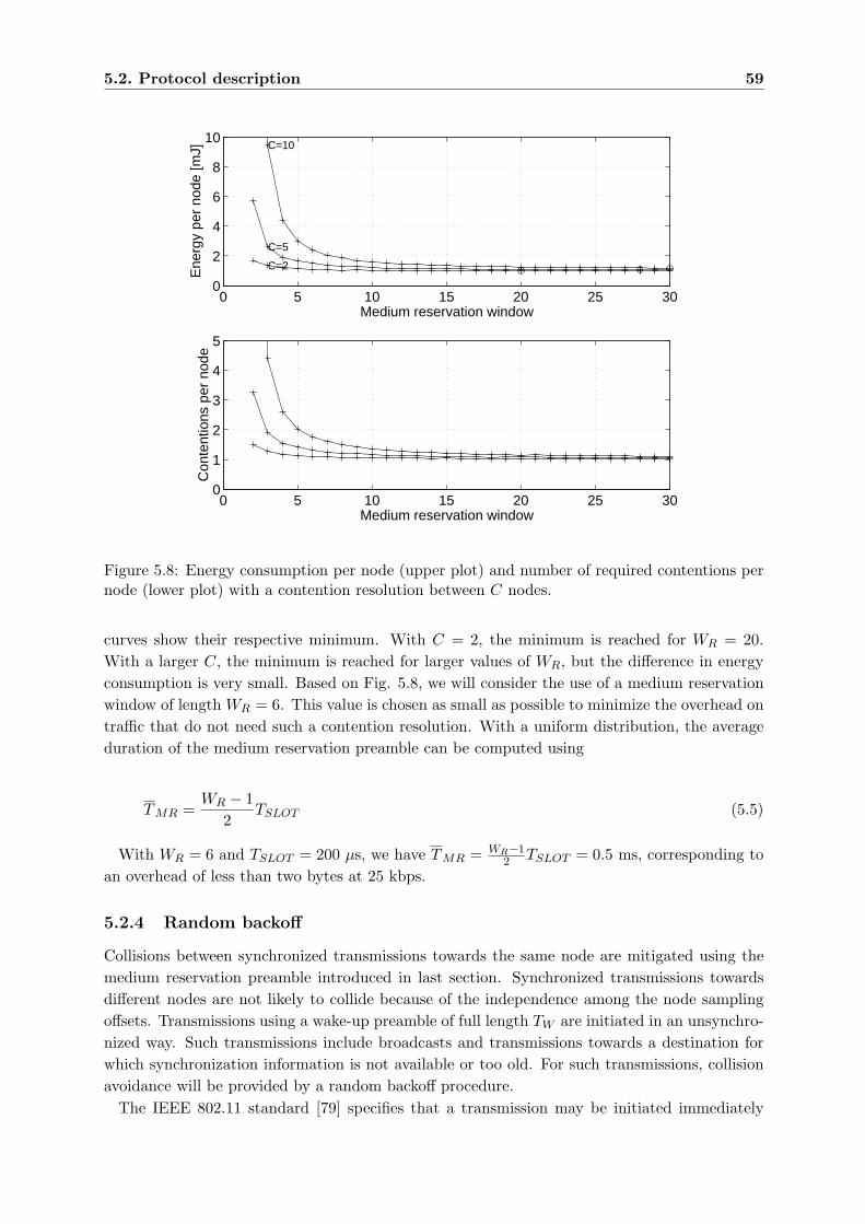
5.2. Protocol description 59
0 5 10 15 20 25 300
2
4
6
8
10
Ene
rgy
per
node
[mJ]
Medium reservation window
C=2
C=5
C=10
0 5 10 15 20 25 300
1
2
3
4
5
Con
tent
ions
per
nod
e
Medium reservation window
Figure 5.8: Energy consumption per node (upper plot) and number of required contentions pernode (lower plot) with a contention resolution between C nodes.
curves show their respective minimum. With C = 2, the minimum is reached for WR = 20.With a larger C, the minimum is reached for larger values of WR, but the difference in energyconsumption is very small. Based on Fig. 5.8, we will consider the use of a medium reservationwindow of length WR = 6. This value is chosen as small as possible to minimize the overhead ontraffic that do not need such a contention resolution. With a uniform distribution, the averageduration of the medium reservation preamble can be computed using
TMR =WR − 1
2TSLOT (5.5)
With WR = 6 and TSLOT = 200 µs, we have TMR = WR−12 TSLOT = 0.5 ms, corresponding to
an overhead of less than two bytes at 25 kbps.
5.2.4 Random backoff
Collisions between synchronized transmissions towards the same node are mitigated using themedium reservation preamble introduced in last section. Synchronized transmissions towardsdifferent nodes are not likely to collide because of the independence among the node samplingoffsets. Transmissions using a wake-up preamble of full length TW are initiated in an unsynchro-nized way. Such transmissions include broadcasts and transmissions towards a destination forwhich synchronization information is not available or too old. For such transmissions, collisionavoidance will be provided by a random backoff procedure.
The IEEE 802.11 standard [79] specifies that a transmission may be initiated immediately
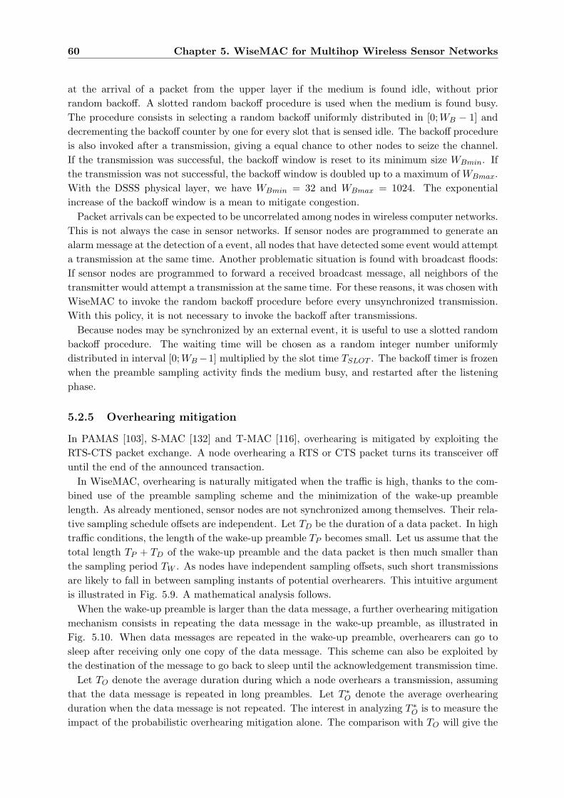
60 Chapter 5. WiseMAC for Multihop Wireless Sensor Networks
at the arrival of a packet from the upper layer if the medium is found idle, without priorrandom backoff. A slotted random backoff procedure is used when the medium is found busy.The procedure consists in selecting a random backoff uniformly distributed in [0;WB − 1] anddecrementing the backoff counter by one for every slot that is sensed idle. The backoff procedureis also invoked after a transmission, giving a equal chance to other nodes to seize the channel.If the transmission was successful, the backoff window is reset to its minimum size WBmin. Ifthe transmission was not successful, the backoff window is doubled up to a maximum of WBmax.With the DSSS physical layer, we have WBmin = 32 and WBmax = 1024. The exponentialincrease of the backoff window is a mean to mitigate congestion.
Packet arrivals can be expected to be uncorrelated among nodes in wireless computer networks.This is not always the case in sensor networks. If sensor nodes are programmed to generate analarm message at the detection of a event, all nodes that have detected some event would attempta transmission at the same time. Another problematic situation is found with broadcast floods:If sensor nodes are programmed to forward a received broadcast message, all neighbors of thetransmitter would attempt a transmission at the same time. For these reasons, it was chosen withWiseMAC to invoke the random backoff procedure before every unsynchronized transmission.With this policy, it is not necessary to invoke the backoff after transmissions.
Because nodes may be synchronized by an external event, it is useful to use a slotted randombackoff procedure. The waiting time will be chosen as a random integer number uniformlydistributed in interval [0;WB−1] multiplied by the slot time TSLOT . The backoff timer is frozenwhen the preamble sampling activity finds the medium busy, and restarted after the listeningphase.
5.2.5 Overhearing mitigation
In PAMAS [103], S-MAC [132] and T-MAC [116], overhearing is mitigated by exploiting theRTS-CTS packet exchange. A node overhearing a RTS or CTS packet turns its transceiver offuntil the end of the announced transaction.
In WiseMAC, overhearing is naturally mitigated when the traffic is high, thanks to the com-bined use of the preamble sampling scheme and the minimization of the wake-up preamblelength. As already mentioned, sensor nodes are not synchronized among themselves. Their rela-tive sampling schedule offsets are independent. Let TD be the duration of a data packet. In hightraffic conditions, the length of the wake-up preamble TP becomes small. Let us assume that thetotal length TP + TD of the wake-up preamble and the data packet is then much smaller thanthe sampling period TW . As nodes have independent sampling offsets, such short transmissionsare likely to fall in between sampling instants of potential overhearers. This intuitive argumentis illustrated in Fig. 5.9. A mathematical analysis follows.
When the wake-up preamble is larger than the data message, a further overhearing mitigationmechanism consists in repeating the data message in the wake-up preamble, as illustrated inFig. 5.10. When data messages are repeated in the wake-up preamble, overhearers can go tosleep after receiving only one copy of the data message. This scheme can also be exploited bythe destination of the message to go back to sleep until the acknowledgement transmission time.
Let TO denote the average duration during which a node overhears a transmission, assumingthat the data message is repeated in long preambles. Let T ∗O denote the average overhearingduration when the data message is not repeated. The interest in analyzing T ∗O is to measure theimpact of the probabilistic overhearing mitigation alone. The comparison with TO will give the
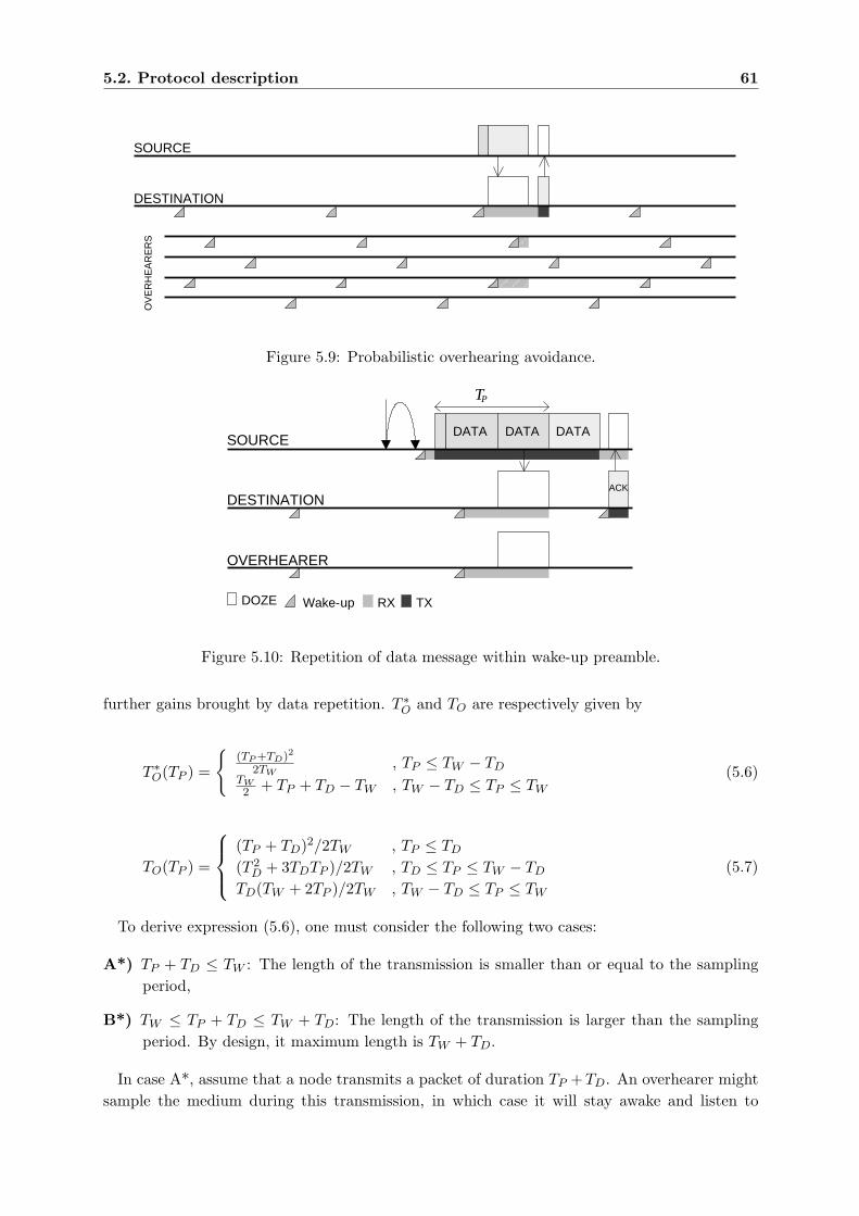
5.2. Protocol description 61
SOURCE
DESTINATION
OV
ER
HE
AR
ER
S
Figure 5.9: Probabilistic overhearing avoidance.
DATA DATA DATA
ACK
TP
DOZE RX TX
DESTINATION
Wake-up
SOURCE
OVERHEARER
Figure 5.10: Repetition of data message within wake-up preamble.
further gains brought by data repetition. T ∗O and TO are respectively given by
T ∗O(TP ) =
{(TP +TD)2
2TW, TP ≤ TW − TD
TW2 + TP + TD − TW , TW − TD ≤ TP ≤ TW
(5.6)
TO(TP ) =
(TP + TD)2/2TW , TP ≤ TD
(T 2D + 3TDTP )/2TW , TD ≤ TP ≤ TW − TD
TD(TW + 2TP )/2TW , TW − TD ≤ TP ≤ TW
(5.7)
To derive expression (5.6), one must consider the following two cases:
A*) TP + TD ≤ TW : The length of the transmission is smaller than or equal to the samplingperiod,
B*) TW ≤ TP + TD ≤ TW + TD: The length of the transmission is larger than the samplingperiod. By design, it maximum length is TW + TD.
In case A*, assume that a node transmits a packet of duration TP +TD. An overhearer mightsample the medium during this transmission, in which case it will stay awake and listen to
62 Chapter 5. WiseMAC for Multihop Wireless Sensor Networks
DATASOURCE
OVERHEARER
TW
TD
YTS
SOURCE
OVERHEARER
TW
TD
YTS
TP
TP
DATADATADATA
A)
B)
C)
SOURCE
OVERHEARER
TW YTS
DATADATADATA DATA
TW
Figure 5.11: Duration of the overhearing period with WiseMAC, when TP < TD (A), TD ≤TP < TW − TD (B) and TW − TD ≤ TP ≤ TW (C).
channel until it becomes idle again. Let Y be the duration during which some node overhears atransmission, where Y ∈ [0;TP +TD]. The sampling period being TW , the transmission will notbe overheard at all with probability TW−TP−TD
TW, i.e. P(Y = 0) = TW−TP−TD
TW. With probability
TP +TDTW
, this node will sample the medium during the transmission, i.e. P(Y > 0) = TP +TDTW
. Y isuniformly distributed over the interval (0;TP + TD], we have P(Y = y) = 1
TWfor Y > 0. Taking
the expectation of the random variable Y , we obtain the average time during which some nodeoverhears a packet not destined to itself Y =
∫ TP +TD
0 y 1TW
dy = (TP +TD)2
2TW.
In case B*, the overhearer will for sure hit the transmission. If the transmission has a lengthTP + TD = TW , the overhearer will listen to it during an average of TW /2 seconds. If thetransmission is longer than that, it will in addition listen to the increment TP + TD − TW .
To derive expression (5.7), one must consider the three following cases (see Fig. 5.11):
A) TP < TD: The wake-up preamble is smaller than a data frame,
B) TD ≤ TP < TW − TD: The wake-up preamble is larger than a data frame. The preambleis filled with copies of the data frame. The total length of the packet TP + TD is smallerthan the sampling period TW ,
C) TW − TD ≤ TP ≤ TW : The total length of the packet TP + TD is larger than the samplingperiod TW . By design, TP must remain smaller than or equal to TW .
In case A, Y is computed identically as in case A*.
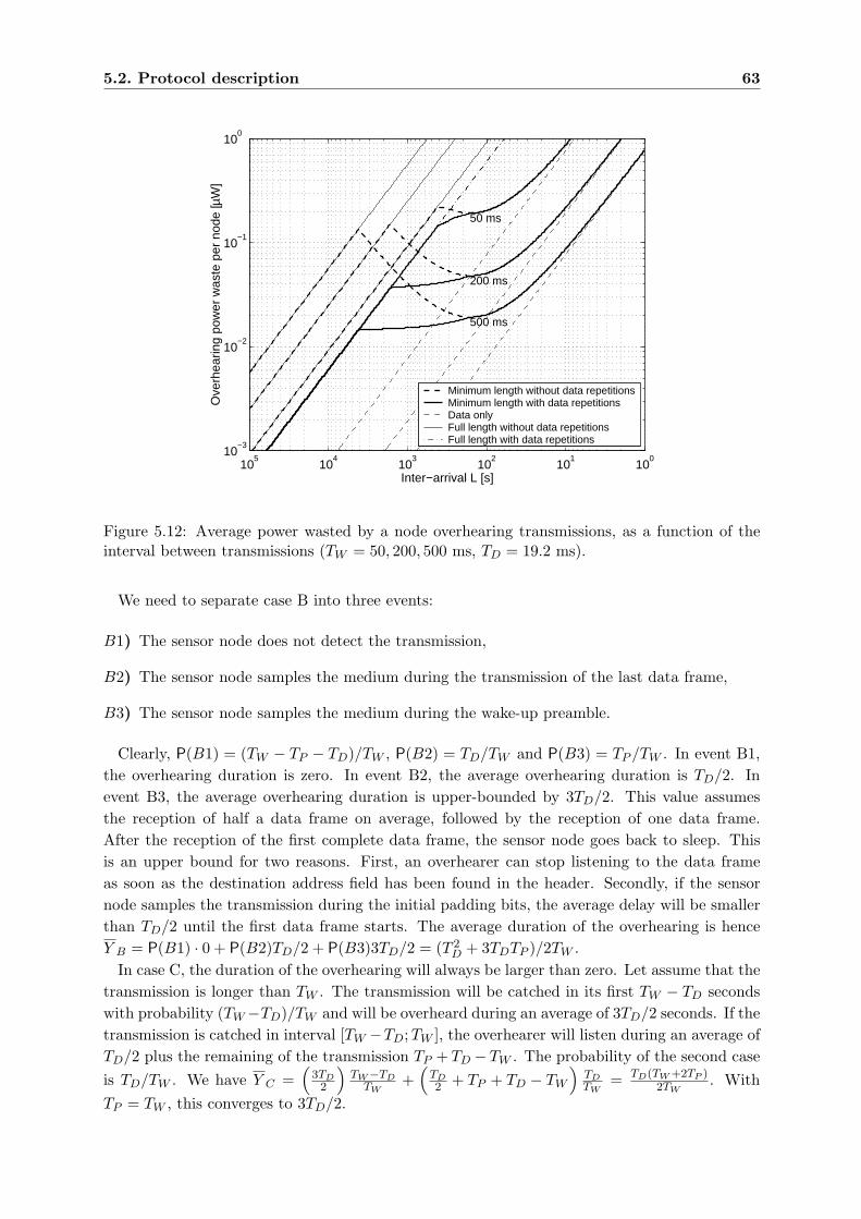
5.2. Protocol description 63
100
101
102
103
104
105
10−3
10−2
10−1
100
50 ms
200 ms
500 ms
Ove
rhea
ring
pow
er w
aste
per
nod
e [µ
W]
Inter−arrival L [s]
Minimum length without data repetitionsMinimum length with data repetitionsData onlyFull length without data repetitionsFull length with data repetitions
Figure 5.12: Average power wasted by a node overhearing transmissions, as a function of theinterval between transmissions (TW = 50, 200, 500 ms, TD = 19.2 ms).
We need to separate case B into three events:
B1) The sensor node does not detect the transmission,
B2) The sensor node samples the medium during the transmission of the last data frame,
B3) The sensor node samples the medium during the wake-up preamble.
Clearly, P(B1) = (TW − TP − TD)/TW , P(B2) = TD/TW and P(B3) = TP /TW . In event B1,the overhearing duration is zero. In event B2, the average overhearing duration is TD/2. Inevent B3, the average overhearing duration is upper-bounded by 3TD/2. This value assumesthe reception of half a data frame on average, followed by the reception of one data frame.After the reception of the first complete data frame, the sensor node goes back to sleep. Thisis an upper bound for two reasons. First, an overhearer can stop listening to the data frameas soon as the destination address field has been found in the header. Secondly, if the sensornode samples the transmission during the initial padding bits, the average delay will be smallerthan TD/2 until the first data frame starts. The average duration of the overhearing is henceY B = P(B1) · 0 + P(B2)TD/2 + P(B3)3TD/2 = (T 2
D + 3TDTP )/2TW .In case C, the duration of the overhearing will always be larger than zero. Let assume that the
transmission is longer than TW . The transmission will be catched in its first TW − TD secondswith probability (TW−TD)/TW and will be overheard during an average of 3TD/2 seconds. If thetransmission is catched in interval [TW −TD;TW ], the overhearer will listen during an average ofTD/2 plus the remaining of the transmission TP + TD − TW . The probability of the second caseis TD/TW . We have Y C =
(3TD
2
)TW−TD
TW+
(TD2 + TP + TD − TW
)TDTW
= TD(TW +2TP )2TW
. WithTP = TW , this converges to 3TD/2.
64 Chapter 5. WiseMAC for Multihop Wireless Sensor Networks
Fig. 5.12 shows the average power wasted by a node due to the overhearing of transmissionsbetween two other nodes, as a function of the interval between these transmissions. The dashedthick line shows T ∗O, the average power overhead caused by overhearing when data messages arenot repeated in the preamble. This overhead is maximized for L = TW /4θ. This maximum isreached for L = 416, 1666, 4166 s for TW = 50, 200, 500 ms respectively. In these cases, it remainsbelow 0.2 µW. The average power overhead is small when L is large, because transmissionscausing such an overhead are rare (as L is large). A power overhead of 0.2 µW per node isnegligible with a network density corresponding to about 10 nodes within reach of a node.With more neighbors, the overhearing overhead can become problematic. In such cases, therepetition of messages within the wake-up preamble, as illustrated in Fig. 5.10, can be usedto further decrease the overhearing overhead. The overhearing overhead TO when consideringthe repetition of data message in the preamble is shown with the solid thick lines in Fig. 5.12.With a small sampling period, the gain over the non-repetition scheme is small. The repetitionscheme becomes powerful when the ratio TW /TD is large. With TW = 200 ms, the powerconsumption overhead is about 4 times smaller for the worst case traffic L = 1666 s. To betterunderstand these curves, Fig. 5.12 also shows the overhearing overhead that would be causedwhen transmitting the data part of the message alone (TP = 0, thin dashed lines) and when thewake-up preamble length is not minimized (thin solid lines when data messages are not repeatedand thin dash-dot line when data messages are repeated in the preamble.).
5.2.6 ”More” bit
An important detail of the WiseMAC protocol, which is also found in the IEEE 802.11 powersave protocol, is the presence of a more bit in the header of data packets. When this bit isset to 1, it indicates that more data packets destined to the same sensor node are waiting inthe buffer of the transmitting node. When a data packet is received with the more bit set, thereceiving sensor node continues to listen after having sent the acknowledgement. The senderwill transmit the following packet right after having received the acknowledgement, withoutinvoking the backoff procedure (see Fig. 5.13). This scheme permits to increase the throughputthat can flow through a given forwarder. The maximum throughput, in packets per seconds, isgiven by the number of buffers available for data frames divided by the sampling period. Aslong as congestion is not reached on the medium, the throughput is hence limited by the sensornode memory size. Another benefit of the more bit scheme is to reduce the end-to-end delay,especially in the event of traffic bursts.
The more bit scheme provides the same functionality as the fragmentation scheme used inS-MAC [132]. An application just needs to segment a large message into smaller packets toobtain the fragmentation behavior. However, the more bit scheme is more flexible. Packets thatdo not belong to the same message but that need to be sent to the same destination will begrouped when using the more bit, while they would be sent individually with the fragmentationscheme.
5.2.7 Inter-frame spaces
Between the end of the data message and the start of the acknowledgement, there is an idleperiod caused by the time needed to turn around the transceiver. The length of this period mustbe specified to allow inter-operability between transceivers with different turn-around times.
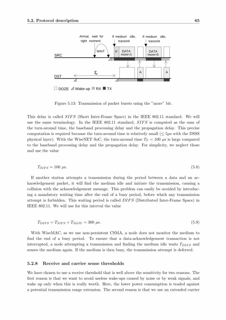
5.2. Protocol description 65
SRC
DST
WAIT
Arrival, wait forright moment
If medium idle,transmit
TWA
DATA
A
P DATAmore=1 more=0
Wake-upDOZE RX TX
If medium idle,transmit
Figure 5.13: Transmission of packet bursts using the ”more” bit.
This delay is called SIFS (Short Inter-Frame Space) in the IEEE 802.11 standard. We willuse the same terminology. In the IEEE 802.11 standard, SIFS is computed as the sum ofthe turn-around time, the baseband processing delay and the propagation delay. This precisecomputation is required because the turn-around time is relatively small (≤ 5µs with the DSSSphysical layer). With the WiseNET SoC, the turn-around time TT = 100 µs is large comparedto the baseband processing delay and the propagation delay. For simplicity, we neglect thoseand use the value
TSIFS = 100 µs. (5.8)
If another station attempts a transmission during the period between a data and an ac-knowledgement packet, it will find the medium idle and initiate the transmission, causing acollision with the acknowledgement message. This problem can easily be avoided by introduc-ing a mandatory waiting time after the end of a busy period, before which any transmissionattempt is forbidden. This waiting period is called DIFS (Distributed Inter-Frame Space) inIEEE 802.11. We will use for this interval the value
TDIFS = TSIFS + TSLOT = 300 µs. (5.9)
With WiseMAC, as we use non-persistent CSMA, a node does not monitor the medium tofind the end of a busy period. To ensure that a data-acknowledgement transaction is notinterrupted, a node attempting a transmission and finding the medium idle waits TDIFS andsenses the medium again. If the medium is then busy, the transmission attempt is deferred.
5.2.8 Receive and carrier sense thresholds
We have chosen to use a receive threshold that is well above the sensitivity for two reasons. Thefirst reason is that we want to avoid useless wake-ups caused by noise or by weak signals, andwake up only when this is really worth. Here, the lower power consumption is traded againsta potential transmission range extension. The second reason is that we use an extended carrier
66 Chapter 5. WiseMAC for Multihop Wireless Sensor Networks
sense range to mitigate the hidden node effect.The classical approach to mitigate the hidden node effect is to use the request to send (RTS)
- clear to send (CTS) dialog before the transmission of the data packet [53, 79]. As the CTSmessage can be heard by all potential interferers, they remain silent during the data transmissionphase. In sensor networks, as the size of data packets is not necessarily larger than signallingmessages, the applicability of this approach is questionable. In any case, with WiseMAC, RTSand CTS messages should have a length of TW seconds to be received by everyone. The resultinglarge overhead clearly forbids using RTS-CTS reservation messages.
An alternative approach to mitigate the hidden node effect consists in using a carrier sensingrange that is larger than the receiver range, such that potential interferers to the destinationwill be englobed in the sensed area. Let PCS and PRMin be respectively the carrier sensing andthe receive thresholds.
The received power PR at the input of the radio receiver can be computed from the power atthe output of the radio transmitter PT using
PR = PT − LT − LP − LR (5.10)
where LT is the loss introduced by the antenna and the radio frequency components on thetransmit path, LR is the loss introduced by the antenna and the radio frequency components onthe receive path and LP the path loss. We assume an antenna loss of 2 dB. Such performanceis for example achieved with 1/4λ low cost and small size (2.8 x 1.3 cm) planar antennas fromAntenna Factor Inc. [48]. The total losses on the transmit path (caused by the antenna and aspurious emission filter) is assumed to be LT = 5 dB. Losses on the receive path (caused by theantenna, an antenna switch and an interference filter) is assumed to be of LR = 7 dB.
For the path loss LP , we consider the classical one-slope model [100, 67]:
LP (d) = L0 + 10α log d (5.11)
where L0 = 20 · log(4π · 868 · 106/3 · 108) = 31 dB is the free space loss at 1 meter and α isthe power decay index. Using this model, the carrier sensing and receive ranges become
dCS = 10PT−LT−LR−L0−PCS
10α (5.12)
and
dR = 10PT−LT−LR−L0−PRMin
10α (5.13)
A signal is assumed to be received without error as long as the ratio between the wanted signaland the sum of interfering signals is above a given SNR. Assuming that the transmitter of thewanted signal is at the receive range dR, the distance at which a single interference should belocated to have the desired signal-to-noise ratio is given by
dI = dR10SNR10α (5.14)
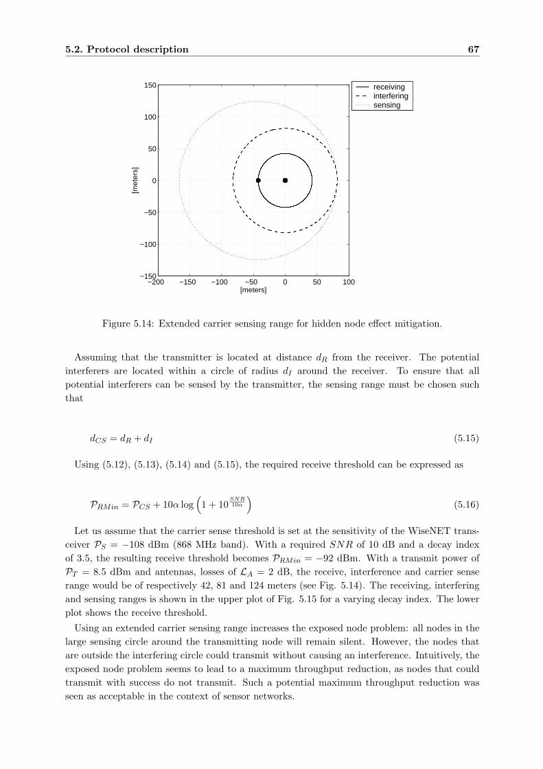
5.2. Protocol description 67
−200 −150 −100 −50 0 50 100−150
−100
−50
0
50
100
150
[meters]
[met
ers]
receivinginterferingsensing
Figure 5.14: Extended carrier sensing range for hidden node effect mitigation.
Assuming that the transmitter is located at distance dR from the receiver. The potentialinterferers are located within a circle of radius dI around the receiver. To ensure that allpotential interferers can be sensed by the transmitter, the sensing range must be chosen suchthat
dCS = dR + dI (5.15)
Using (5.12), (5.13), (5.14) and (5.15), the required receive threshold can be expressed as
PRMin = PCS + 10α log(1 + 10
SNR10α
)(5.16)
Let us assume that the carrier sense threshold is set at the sensitivity of the WiseNET trans-ceiver PS = −108 dBm (868 MHz band). With a required SNR of 10 dB and a decay indexof 3.5, the resulting receive threshold becomes PRMin = −92 dBm. With a transmit power ofPT = 8.5 dBm and antennas, losses of LA = 2 dB, the receive, interference and carrier senserange would be of respectively 42, 81 and 124 meters (see Fig. 5.14). The receiving, interferingand sensing ranges is shown in the upper plot of Fig. 5.15 for a varying decay index. The lowerplot shows the receive threshold.
Using an extended carrier sensing range increases the exposed node problem: all nodes in thelarge sensing circle around the transmitting node will remain silent. However, the nodes thatare outside the interfering circle could transmit without causing an interference. Intuitively, theexposed node problem seems to lead to a maximum throughput reduction, as nodes that couldtransmit with success do not transmit. Such a potential maximum throughput reduction wasseen as acceptable in the context of sensor networks.
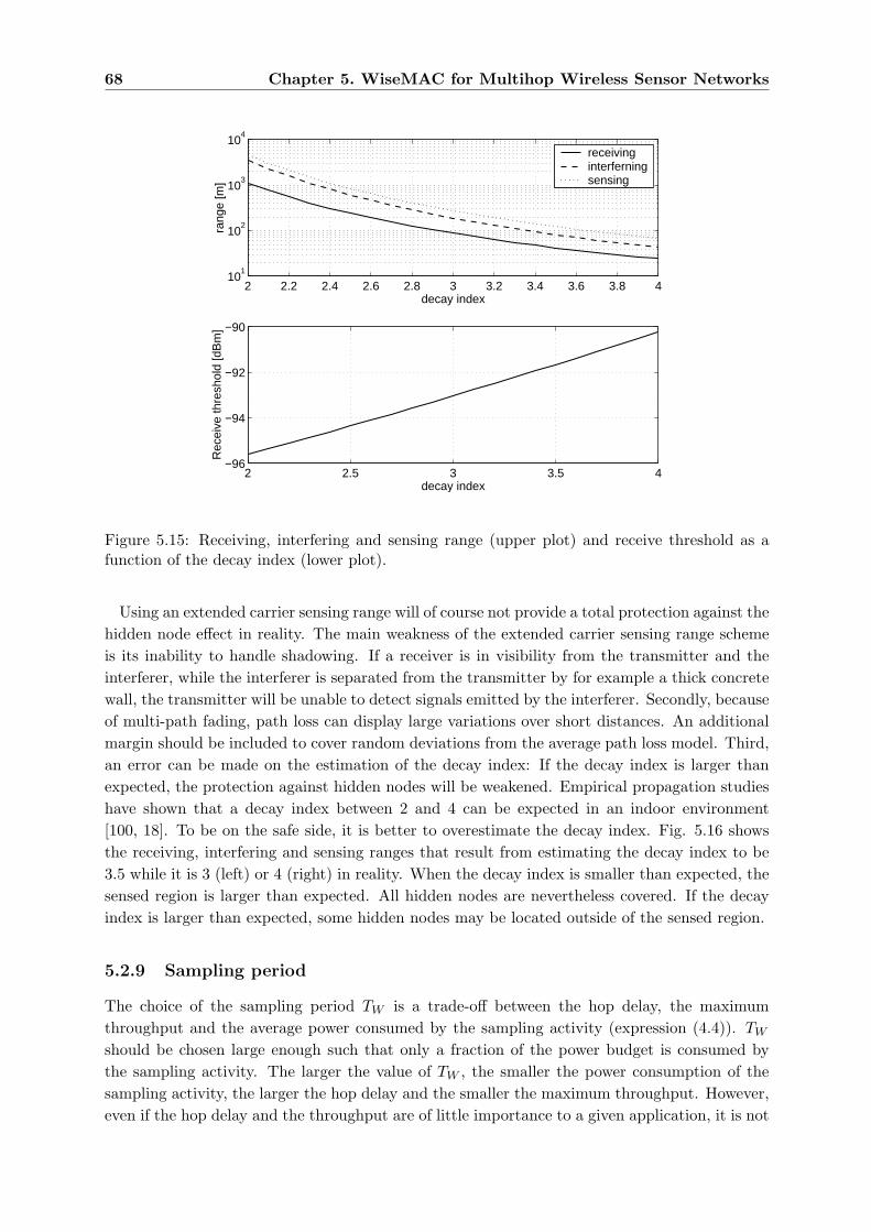
68 Chapter 5. WiseMAC for Multihop Wireless Sensor Networks
2 2.2 2.4 2.6 2.8 3 3.2 3.4 3.6 3.8 410
1
102
103
104
decay index
rang
e [m
]
receivinginterferningsensing
2 2.5 3 3.5 4−96
−94
−92
−90
decay index
Rec
eive
thre
shol
d [d
Bm
]
Figure 5.15: Receiving, interfering and sensing range (upper plot) and receive threshold as afunction of the decay index (lower plot).
Using an extended carrier sensing range will of course not provide a total protection against thehidden node effect in reality. The main weakness of the extended carrier sensing range schemeis its inability to handle shadowing. If a receiver is in visibility from the transmitter and theinterferer, while the interferer is separated from the transmitter by for example a thick concretewall, the transmitter will be unable to detect signals emitted by the interferer. Secondly, becauseof multi-path fading, path loss can display large variations over short distances. An additionalmargin should be included to cover random deviations from the average path loss model. Third,an error can be made on the estimation of the decay index: If the decay index is larger thanexpected, the protection against hidden nodes will be weakened. Empirical propagation studieshave shown that a decay index between 2 and 4 can be expected in an indoor environment[100, 18]. To be on the safe side, it is better to overestimate the decay index. Fig. 5.16 showsthe receiving, interfering and sensing ranges that result from estimating the decay index to be3.5 while it is 3 (left) or 4 (right) in reality. When the decay index is smaller than expected, thesensed region is larger than expected. All hidden nodes are nevertheless covered. If the decayindex is larger than expected, some hidden nodes may be located outside of the sensed region.
5.2.9 Sampling period
The choice of the sampling period TW is a trade-off between the hop delay, the maximumthroughput and the average power consumed by the sampling activity (expression (4.4)). TW
should be chosen large enough such that only a fraction of the power budget is consumed bythe sampling activity. The larger the value of TW , the smaller the power consumption of thesampling activity, the larger the hop delay and the smaller the maximum throughput. However,even if the hop delay and the throughput are of little importance to a given application, it is not

5.3. Performance analysis 69
−400 −300 −200 −100 0 100 200−300
−200
−100
0
100
200
300
[meters]
[met
ers]
−100 −50 0 50−80
−60
−40
−20
0
20
40
60
80
[meters]
[met
ers]
Figure 5.16: Effect of a wrong estimation of the decay index. The estimated decay index usedto compute the receive threshold is equal to 3.5 in both cases. The effective decay index is equalto 3 on the left plot, and to 4 and the right plot.
0 100 200 300 400 500 600 700 800 900 10000123456789
10
TW
[ms]
Life
time
[yea
rs]
Figure 5.17: Lifetime when sampling the medium with period TW (no traffic).
interesting, in terms of lifetime, and when using an alkaline battery, to have a power consumptionfor the sampling activity that is negligible compared to the leaked power. Fig. 5.17 shows theexpected lifetime of a sensor node as a function of the sampling period TW . From this plot,it can be seen that a good value for the sampling period when using the WiseNET transceiverwith an alkaline battery is TW = 100 ms, which results in a power consumption of the samplingactivity of (PSTS + PRTI)/TW = 8.8 µW. Using a larger value for TW increases linearly thedelay and decreases linearly the maximum throughput without increasing the lifetime much.
5.3 Performance analysis
The performance of the WiseMAC protocol is analyzed through simulation and theoreticalcalculations. Comparisons are made with S-MAC, T-MAC, CSMA/CA and an ideal protocol.Models of S-MAC and T-MAC were not available on the used simulation platform. A CSMA
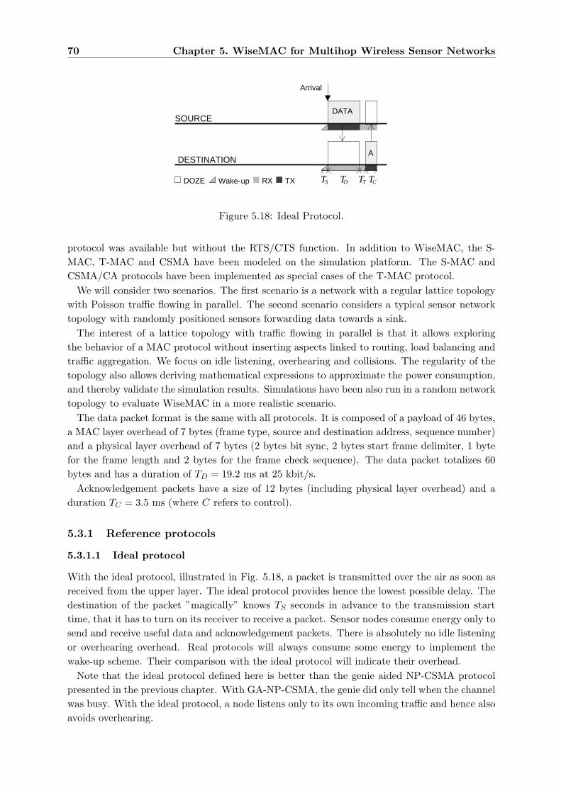
70 Chapter 5. WiseMAC for Multihop Wireless Sensor Networks
SOURCE
DESTINATIONA
Arrival
DATA
TD TCTTTSDOZE RX TXWake-up
Figure 5.18: Ideal Protocol.
protocol was available but without the RTS/CTS function. In addition to WiseMAC, the S-MAC, T-MAC and CSMA have been modeled on the simulation platform. The S-MAC andCSMA/CA protocols have been implemented as special cases of the T-MAC protocol.
We will consider two scenarios. The first scenario is a network with a regular lattice topologywith Poisson traffic flowing in parallel. The second scenario considers a typical sensor networktopology with randomly positioned sensors forwarding data towards a sink.
The interest of a lattice topology with traffic flowing in parallel is that it allows exploringthe behavior of a MAC protocol without inserting aspects linked to routing, load balancing andtraffic aggregation. We focus on idle listening, overhearing and collisions. The regularity of thetopology also allows deriving mathematical expressions to approximate the power consumption,and thereby validate the simulation results. Simulations have been also run in a random networktopology to evaluate WiseMAC in a more realistic scenario.
The data packet format is the same with all protocols. It is composed of a payload of 46 bytes,a MAC layer overhead of 7 bytes (frame type, source and destination address, sequence number)and a physical layer overhead of 7 bytes (2 bytes bit sync, 2 bytes start frame delimiter, 1 bytefor the frame length and 2 bytes for the frame check sequence). The data packet totalizes 60bytes and has a duration of TD = 19.2 ms at 25 kbit/s.
Acknowledgement packets have a size of 12 bytes (including physical layer overhead) and aduration TC = 3.5 ms (where C refers to control).
5.3.1 Reference protocols
5.3.1.1 Ideal protocol
With the ideal protocol, illustrated in Fig. 5.18, a packet is transmitted over the air as soon asreceived from the upper layer. The ideal protocol provides hence the lowest possible delay. Thedestination of the packet ”magically” knows TS seconds in advance to the transmission starttime, that it has to turn on its receiver to receive a packet. Sensor nodes consume energy only tosend and receive useful data and acknowledgement packets. There is absolutely no idle listeningor overhearing overhead. Real protocols will always consume some energy to implement thewake-up scheme. Their comparison with the ideal protocol will indicate their overhead.
Note that the ideal protocol defined here is better than the genie aided NP-CSMA protocolpresented in the previous chapter. With GA-NP-CSMA, the genie did only tell when the channelwas busy. With the ideal protocol, a node listens only to its own incoming traffic and hence alsoavoids overhearing.
5.3. Performance analysis 71
5.3.1.2 S-MAC
The S-MAC protocol, already introduced in section 2.3.5, defines sleep intervals, in which all thenodes of the network sleep, and active intervals, in which nodes synchronize and/or can demandto their neighbors to remain awake and receive a transmission [132]. The sum of both intervalsis called a frame. The active interval is composed of a phase during which nodes listen for SYNCpackets and a phase during which nodes listen for RTS and CTS packets. For fair comparisonwith WiseMAC, we consider only a phase during which nodes listen for RTS and CTS packets.As SYNC packets are exchanged only sporadically, they may well be transmitted in competitionto RTS packets. As illustrated in Fig. 5.19, the listen interval should be long enough for thelongest possible backoff followed by an RTS-CTS packet exchange. In the simulation model,the synchronization mechanism has not been implemented. Instead, the network is assumedto be always perfectly synchronized. The model represents an idealized version of S-MAC.The performance results are in this sense an upper bound of what can be obtained with areal implementation of S-MAC that would have to exchange signalling packets to maintain thesynchronization.
With S-MAC, one must choose the size of the backoff window as small as possible to minimizethe average power consumption. The backoff should however be chosen large enough to avoidcollisions with high probability. As proposed in [133], we will use WB = 32. The longest possiblecontention duration is then (WB − 1)TSLOT = 6.2 ms. After the backoff waiting time, clearchannel assessment is repeated two times at an interval of TDIFS = 0.3 ms. In the simulationmodel, RTS and CTS packets have both a size of 12 bytes (including physical overhead) and aduration of TRTS = TCTS = 3.5 ms at 25 kbps. The minimum duration of the listen intervalis hence chosen to be TL = (WB − 1)TSLOT + TDIFS + TRTS + TT + TCTS = 31 · 0.2 + 0.3 +3.5 + 0.1 + 3.5 = 14 ms. If two nodes exchange successfully an RTS and CTS packet during thelisten interval, they remain active until the end of the data and acknowledgement transmissions.Other nodes overhearing these RTS and CTS packets update their virtual carrier sense NAVvector and go to sleep.
A listen time of 115 ms was used on the Mica motes implementation of S-MAC [133]. This is8 times more that what we selected here. At 10% duty cycle, this results in a frame duration of1.15 ms which results is quite large hop delays. The reason of this larger listen interval stemsfrom the additional period reserved for synchronization packets and from the lower bit effectivebit rate (10 kbps after Manchester decoding on the Mica motes compared to 25 kbps in thissimulation). The listen interval chosen here provides much better results and permits a faircomparison of S-MAC with WiseMAC. Note that with a shorter listen interval, the problemof keeping the network sufficiently synchronized becomes more difficult, and that the cost ofmaintaining the synchronization has been neglected with S-MAC.
Three different frame durations will be considered: TF = 1400, 280 and 140 ms, providinga duty cycle of 1, 5 and 10% in the absence of traffic (10% is the default duty cycle in theimplementation of S-MAC on the motes [131]).
5.3.1.3 T-MAC
The T-MAC protocol [116], already introduced in section 2.3.5, is an improved version of S-MAC. The difference is that the duration of the active period is dynamically adapted to thetraffic, using a timeout. The active period is ended whenever physical and virtual carrier sensing
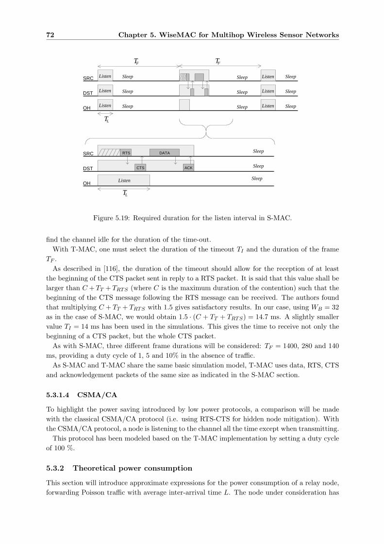
72 Chapter 5. WiseMAC for Multihop Wireless Sensor Networks
SRC RTS
CTS
DATA
ACKDST
OHSleepListen
Sleep
Sleep
TL
TF
SRC
DST
OH SleepListen Sleep Sleep
SleepListen Sleep Sleep
SleepListen Sleep Sleep
Listen
Listen
Listen
TL
TF
Figure 5.19: Required duration for the listen interval in S-MAC.
find the channel idle for the duration of the time-out.With T-MAC, one must select the duration of the timeout TI and the duration of the frame
TF .As described in [116], the duration of the timeout should allow for the reception of at least
the beginning of the CTS packet sent in reply to a RTS packet. It is said that this value shall belarger than C + TT + TRTS (where C is the maximum duration of the contention) such that thebeginning of the CTS message following the RTS message can be received. The authors foundthat multiplying C + TT + TRTS with 1.5 gives satisfactory results. In our case, using WB = 32as in the case of S-MAC, we would obtain 1.5 · (C + TT + TRTS) = 14.7 ms. A slightly smallervalue TI = 14 ms has been used in the simulations. This gives the time to receive not only thebeginning of a CTS packet, but the whole CTS packet.
As with S-MAC, three different frame durations will be considered: TF = 1400, 280 and 140ms, providing a duty cycle of 1, 5 and 10% in the absence of traffic.
As S-MAC and T-MAC share the same basic simulation model, T-MAC uses data, RTS, CTSand acknowledgement packets of the same size as indicated in the S-MAC section.
5.3.1.4 CSMA/CA
To highlight the power saving introduced by low power protocols, a comparison will be madewith the classical CSMA/CA protocol (i.e. using RTS-CTS for hidden node mitigation). Withthe CSMA/CA protocol, a node is listening to the channel all the time except when transmitting.
This protocol has been modeled based on the T-MAC implementation by setting a duty cycleof 100 %.
5.3.2 Theoretical power consumption
This section will introduce approximate expressions for the power consumption of a relay node,forwarding Poisson traffic with average inter-arrival time L. The node under consideration has
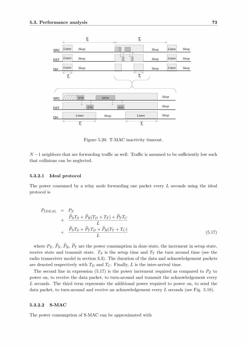
5.3. Performance analysis 73
SRC RTS
CTS
DATA
ACKDST
OH SleepListen Listen Sleep
Sleep
Sleep
TI TI
TF
SRC
DST
OH SleepListen Sleep Sleep
SleepListen Sleep Sleep
SleepListen Sleep Sleep
Listen
Listen
Listen
TITI
TF
Figure 5.20: T-MAC inactivity timeout.
N −1 neighbors that are forwarding traffic as well. Traffic is assumed to be sufficiently low suchthat collisions can be neglected.
5.3.2.1 Ideal protocol
The power consumed by a relay node forwarding one packet every L seconds using the idealprotocol is
PIDEAL = PZ
+PSTS + PR(TD + TT ) + PT TC
L
+PSTS + PT TD + PR(TT + TC)
L(5.17)
where PZ , PS , PR, PT are the power consumption in doze state, the increment in setup state,receive state and transmit state. TS is the setup time and TT the turn around time (see theradio transceiver model in section 3.3). The duration of the data and acknowledgement packetsare denoted respectively with TD and TC . Finally, L is the inter-arrival time.
The second line in expression (5.17) is the power increment required as compared to PZ topower on, to receive the data packet, to turn-around and transmit the acknowledgement everyL seconds. The third term represents the additional power required to power on, to send thedata packet, to turn-around and receive an acknowledgement every L seconds (see Fig. 5.18).
5.3.2.2 S-MAC
The power consumption of S-MAC can be approximated with
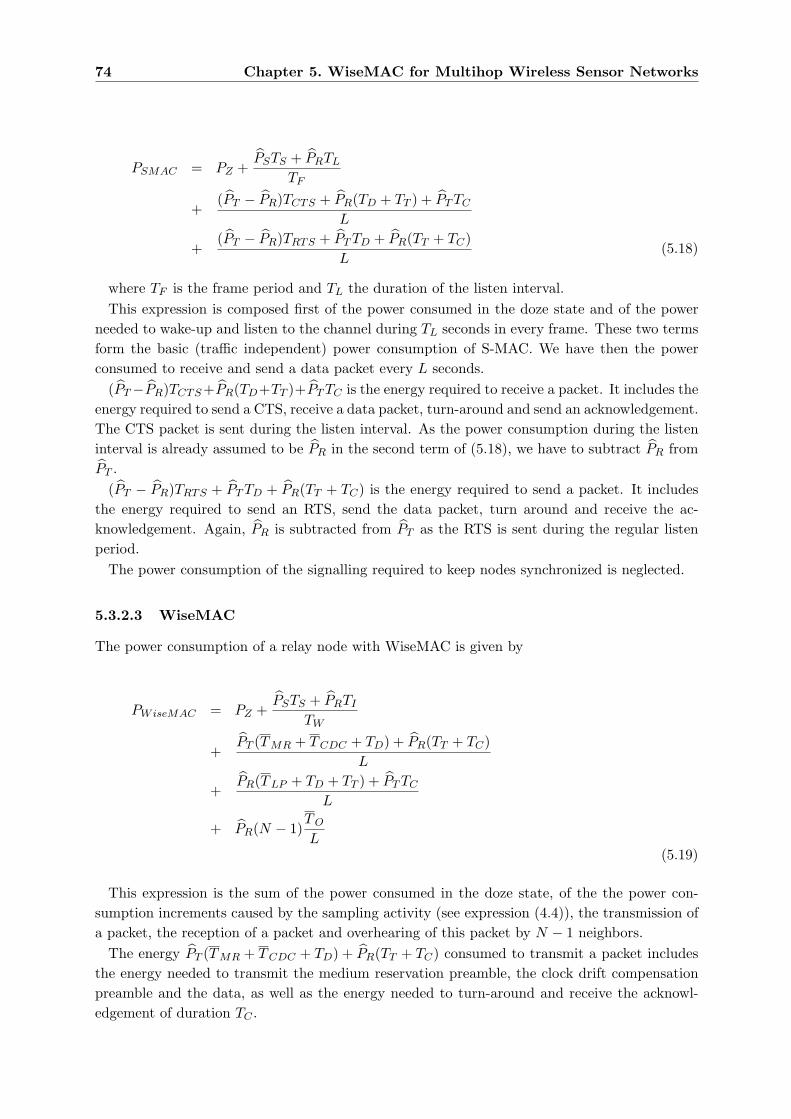
74 Chapter 5. WiseMAC for Multihop Wireless Sensor Networks
PSMAC = PZ +PSTS + PRTL
TF
+(PT − PR)TCTS + PR(TD + TT ) + PT TC
L
+(PT − PR)TRTS + PT TD + PR(TT + TC)
L(5.18)
where TF is the frame period and TL the duration of the listen interval.This expression is composed first of the power consumed in the doze state and of the power
needed to wake-up and listen to the channel during TL seconds in every frame. These two termsform the basic (traffic independent) power consumption of S-MAC. We have then the powerconsumed to receive and send a data packet every L seconds.
(PT−PR)TCTS+PR(TD+TT )+PT TC is the energy required to receive a packet. It includes theenergy required to send a CTS, receive a data packet, turn-around and send an acknowledgement.The CTS packet is sent during the listen interval. As the power consumption during the listeninterval is already assumed to be PR in the second term of (5.18), we have to subtract PR fromPT .
(PT − PR)TRTS + PT TD + PR(TT + TC) is the energy required to send a packet. It includesthe energy required to send an RTS, send the data packet, turn around and receive the ac-knowledgement. Again, PR is subtracted from PT as the RTS is sent during the regular listenperiod.
The power consumption of the signalling required to keep nodes synchronized is neglected.
5.3.2.3 WiseMAC
The power consumption of a relay node with WiseMAC is given by
PWiseMAC = PZ +PSTS + PRTI
TW
+PT (TMR + TCDC + TD) + PR(TT + TC)
L
+PR(TLP + TD + TT ) + PT TC
L
+ PR(N − 1)TO
L(5.19)
This expression is the sum of the power consumed in the doze state, of the the power con-sumption increments caused by the sampling activity (see expression (4.4)), the transmission ofa packet, the reception of a packet and overhearing of this packet by N − 1 neighbors.
The energy PT (TMR + TCDC + TD) + PR(TT + TC) consumed to transmit a packet includesthe energy needed to transmit the medium reservation preamble, the clock drift compensationpreamble and the data, as well as the energy needed to turn-around and receive the acknowl-edgement of duration TC .
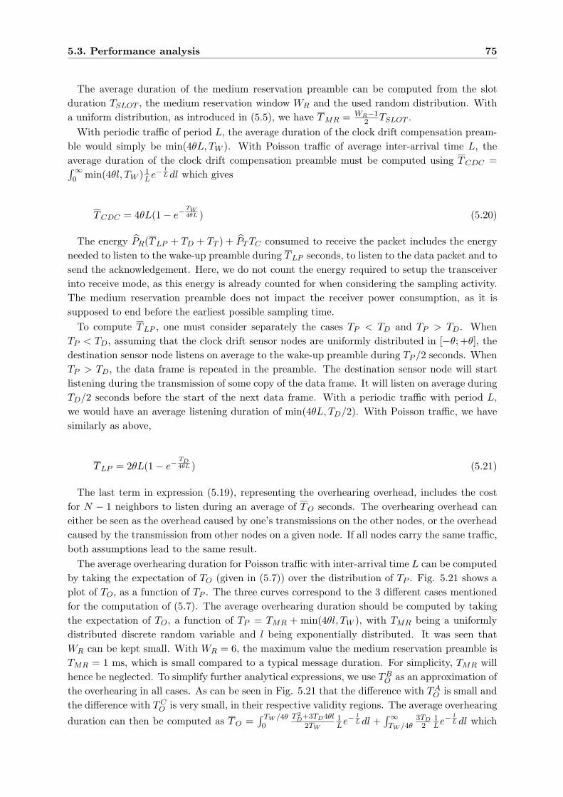
5.3. Performance analysis 75
The average duration of the medium reservation preamble can be computed from the slotduration TSLOT , the medium reservation window WR and the used random distribution. Witha uniform distribution, as introduced in (5.5), we have TMR = WR−1
2 TSLOT .With periodic traffic of period L, the average duration of the clock drift compensation pream-
ble would simply be min(4θL, TW ). With Poisson traffic of average inter-arrival time L, theaverage duration of the clock drift compensation preamble must be computed using TCDC =∫∞0 min(4θl, TW ) 1
Le−lL dl which gives
TCDC = 4θL(1− e−TW4θL ) (5.20)
The energy PR(TLP + TD + TT ) + PT TC consumed to receive the packet includes the energyneeded to listen to the wake-up preamble during TLP seconds, to listen to the data packet and tosend the acknowledgement. Here, we do not count the energy required to setup the transceiverinto receive mode, as this energy is already counted for when considering the sampling activity.The medium reservation preamble does not impact the receiver power consumption, as it issupposed to end before the earliest possible sampling time.
To compute TLP , one must consider separately the cases TP < TD and TP > TD. WhenTP < TD, assuming that the clock drift sensor nodes are uniformly distributed in [−θ; +θ], thedestination sensor node listens on average to the wake-up preamble during TP /2 seconds. WhenTP > TD, the data frame is repeated in the preamble. The destination sensor node will startlistening during the transmission of some copy of the data frame. It will listen on average duringTD/2 seconds before the start of the next data frame. With a periodic traffic with period L,we would have an average listening duration of min(4θL, TD/2). With Poisson traffic, we havesimilarly as above,
TLP = 2θL(1− e−TD4θL ) (5.21)
The last term in expression (5.19), representing the overhearing overhead, includes the costfor N − 1 neighbors to listen during an average of TO seconds. The overhearing overhead caneither be seen as the overhead caused by one’s transmissions on the other nodes, or the overheadcaused by the transmission from other nodes on a given node. If all nodes carry the same traffic,both assumptions lead to the same result.
The average overhearing duration for Poisson traffic with inter-arrival time L can be computedby taking the expectation of TO (given in (5.7)) over the distribution of TP . Fig. 5.21 shows aplot of TO, as a function of TP . The three curves correspond to the 3 different cases mentionedfor the computation of (5.7). The average overhearing duration should be computed by takingthe expectation of TO, a function of TP = TMR + min(4θl, TW ), with TMR being a uniformlydistributed discrete random variable and l being exponentially distributed. It was seen thatWR can be kept small. With WR = 6, the maximum value the medium reservation preamble isTMR = 1 ms, which is small compared to a typical message duration. For simplicity, TMR willhence be neglected. To simplify further analytical expressions, we use TB
O as an approximation ofthe overhearing in all cases. As can be seen in Fig. 5.21 that the difference with TA
O is small andthe difference with TC
O is very small, in their respective validity regions. The average overhearing
duration can then be computed as TO =∫ TW /4θ0
T 2D+3TD4θl
2TW
1Le−
lL dl +
∫∞TW /4θ
3TD2
1Le−
lL dl which
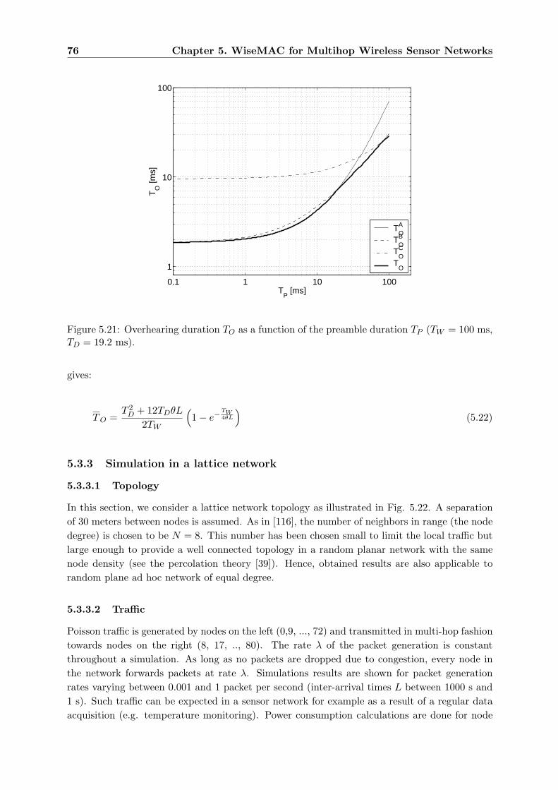
76 Chapter 5. WiseMAC for Multihop Wireless Sensor Networks
0.1 1 10 100
1
10
100
TP [ms]
TO
[ms]
TOA
TOB
TOC
TO
Figure 5.21: Overhearing duration TO as a function of the preamble duration TP (TW = 100 ms,TD = 19.2 ms).
gives:
TO =T 2
D + 12TDθL
2TW
(1− e−
TW4θL
)(5.22)
5.3.3 Simulation in a lattice network
5.3.3.1 Topology
In this section, we consider a lattice network topology as illustrated in Fig. 5.22. A separationof 30 meters between nodes is assumed. As in [116], the number of neighbors in range (the nodedegree) is chosen to be N = 8. This number has been chosen small to limit the local traffic butlarge enough to provide a well connected topology in a random planar network with the samenode density (see the percolation theory [39]). Hence, obtained results are also applicable torandom plane ad hoc network of equal degree.
5.3.3.2 Traffic
Poisson traffic is generated by nodes on the left (0,9, ..., 72) and transmitted in multi-hop fashiontowards nodes on the right (8, 17, .., 80). The rate λ of the packet generation is constantthroughout a simulation. As long as no packets are dropped due to congestion, every node inthe network forwards packets at rate λ. Simulations results are shown for packet generationrates varying between 0.001 and 1 packet per second (inter-arrival times L between 1000 s and1 s). Such traffic can be expected in a sensor network for example as a result of a regular dataacquisition (e.g. temperature monitoring). Power consumption calculations are done for node
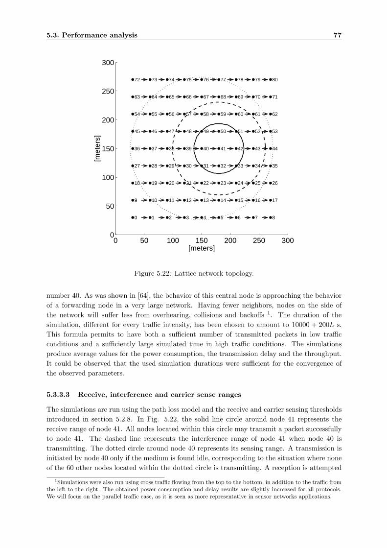
5.3. Performance analysis 77
0 50 100 150 200 250 3000
50
100
150
200
250
300
0 1 2 3 4 5 6 7 8
9 10 11 12 13 14 15 16 17
18 19 20 21 22 23 24 25 26
27 28 29 30 31 32 33 34 35
36 37 38 39 40 41 42 43 44
45 46 47 48 49 50 51 52 53
54 55 56 57 58 59 60 61 62
63 64 65 66 67 68 69 70 71
72 73 74 75 76 77 78 79 80
[meters]
[met
ers]
Figure 5.22: Lattice network topology.
number 40. As was shown in [64], the behavior of this central node is approaching the behaviorof a forwarding node in a very large network. Having fewer neighbors, nodes on the side ofthe network will suffer less from overhearing, collisions and backoffs 1. The duration of thesimulation, different for every traffic intensity, has been chosen to amount to 10000 + 200L s.This formula permits to have both a sufficient number of transmitted packets in low trafficconditions and a sufficiently large simulated time in high traffic conditions. The simulationsproduce average values for the power consumption, the transmission delay and the throughput.It could be observed that the used simulation durations were sufficient for the convergence ofthe observed parameters.
5.3.3.3 Receive, interference and carrier sense ranges
The simulations are run using the path loss model and the receive and carrier sensing thresholdsintroduced in section 5.2.8. In Fig. 5.22, the solid line circle around node 41 represents thereceive range of node 41. All nodes located within this circle may transmit a packet successfullyto node 41. The dashed line represents the interference range of node 41 when node 40 istransmitting. The dotted circle around node 40 represents its sensing range. A transmission isinitiated by node 40 only if the medium is found idle, corresponding to the situation where noneof the 60 other nodes located within the dotted circle is transmitting. A reception is attempted
1Simulations were also run using cross traffic flowing from the top to the bottom, in addition to the traffic fromthe left to the right. The obtained power consumption and delay results are slightly increased for all protocols.We will focus on the parallel traffic case, as it is seen as more representative in sensor networks applications.
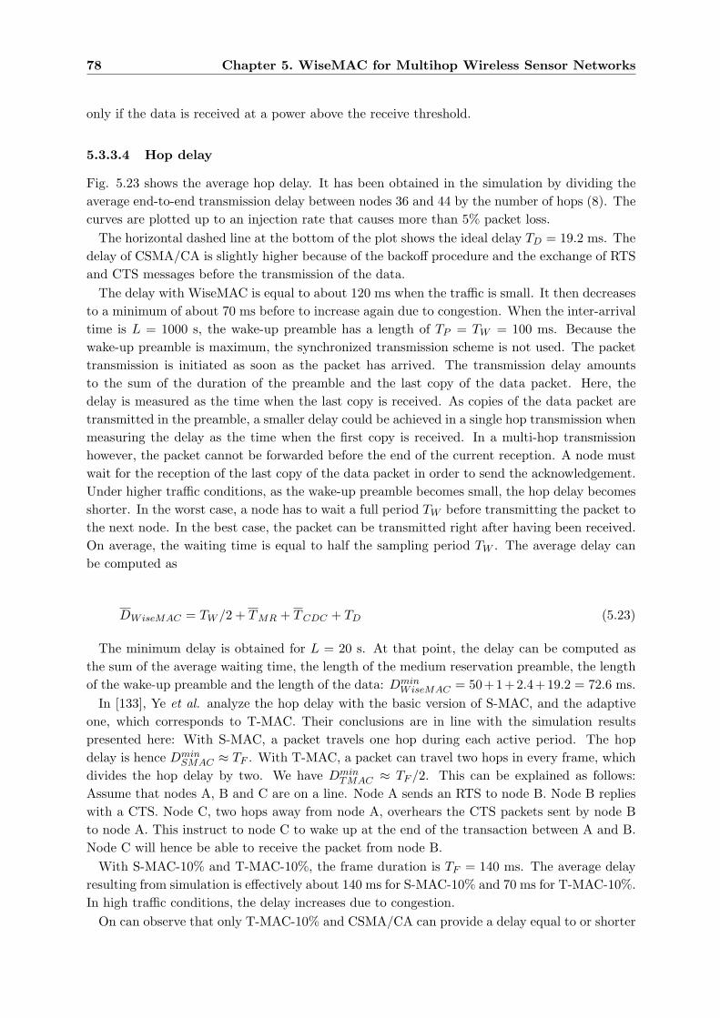
78 Chapter 5. WiseMAC for Multihop Wireless Sensor Networks
only if the data is received at a power above the receive threshold.
5.3.3.4 Hop delay
Fig. 5.23 shows the average hop delay. It has been obtained in the simulation by dividing theaverage end-to-end transmission delay between nodes 36 and 44 by the number of hops (8). Thecurves are plotted up to an injection rate that causes more than 5% packet loss.
The horizontal dashed line at the bottom of the plot shows the ideal delay TD = 19.2 ms. Thedelay of CSMA/CA is slightly higher because of the backoff procedure and the exchange of RTSand CTS messages before the transmission of the data.
The delay with WiseMAC is equal to about 120 ms when the traffic is small. It then decreasesto a minimum of about 70 ms before to increase again due to congestion. When the inter-arrivaltime is L = 1000 s, the wake-up preamble has a length of TP = TW = 100 ms. Because thewake-up preamble is maximum, the synchronized transmission scheme is not used. The packettransmission is initiated as soon as the packet has arrived. The transmission delay amountsto the sum of the duration of the preamble and the last copy of the data packet. Here, thedelay is measured as the time when the last copy is received. As copies of the data packet aretransmitted in the preamble, a smaller delay could be achieved in a single hop transmission whenmeasuring the delay as the time when the first copy is received. In a multi-hop transmissionhowever, the packet cannot be forwarded before the end of the current reception. A node mustwait for the reception of the last copy of the data packet in order to send the acknowledgement.Under higher traffic conditions, as the wake-up preamble becomes small, the hop delay becomesshorter. In the worst case, a node has to wait a full period TW before transmitting the packet tothe next node. In the best case, the packet can be transmitted right after having been received.On average, the waiting time is equal to half the sampling period TW . The average delay canbe computed as
DWiseMAC = TW /2 + TMR + TCDC + TD (5.23)
The minimum delay is obtained for L = 20 s. At that point, the delay can be computed asthe sum of the average waiting time, the length of the medium reservation preamble, the lengthof the wake-up preamble and the length of the data: Dmin
WiseMAC = 50+1+2.4+19.2 = 72.6 ms.In [133], Ye et al. analyze the hop delay with the basic version of S-MAC, and the adaptive
one, which corresponds to T-MAC. Their conclusions are in line with the simulation resultspresented here: With S-MAC, a packet travels one hop during each active period. The hopdelay is hence Dmin
SMAC ≈ TF . With T-MAC, a packet can travel two hops in every frame, whichdivides the hop delay by two. We have Dmin
TMAC ≈ TF /2. This can be explained as follows:Assume that nodes A, B and C are on a line. Node A sends an RTS to node B. Node B replieswith a CTS. Node C, two hops away from node A, overhears the CTS packets sent by node Bto node A. This instruct to node C to wake up at the end of the transaction between A and B.Node C will hence be able to receive the packet from node B.
With S-MAC-10% and T-MAC-10%, the frame duration is TF = 140 ms. The average delayresulting from simulation is effectively about 140 ms for S-MAC-10% and 70 ms for T-MAC-10%.In high traffic conditions, the delay increases due to congestion.
On can observe that only T-MAC-10% and CSMA/CA can provide a delay equal to or shorter
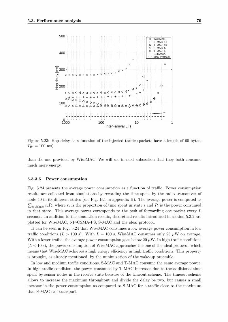
5.3. Performance analysis 79
11010010000
100
200
300
400
500
Hop
del
ay [m
s]
Inter−arrival L [s]
WiseMACS−MAC−10T−MAC−10S−MAC−5T−MAC−5CSMA/CAIdeal Protocol
Figure 5.23: Hop delay as a function of the injected traffic (packets have a length of 60 bytes,TW = 100 ms).
than the one provided by WiseMAC. We will see in next subsection that they both consumemuch more energy.
5.3.3.5 Power consumption
Fig. 5.24 presents the average power consumption as a function of traffic. Power consumptionresults are collected from simulations by recording the time spent by the radio transceiver ofnode 40 in its different states (see Fig. B.1 in appendix B). The average power is computed as∑
i∈States riPi, where ri is the proportion of time spent in state i and Pi is the power consumedin that state. This average power corresponds to the task of forwarding one packet every L
seconds. In addition to the simulation results, theoretical results introduced in section 5.3.2 areplotted for WiseMAC, NP-CSMA-PS, S-MAC and the ideal protocol.
It can be seen in Fig. 5.24 that WiseMAC consumes a low average power consumption in lowtraffic conditions (L > 100 s). With L = 100 s, WiseMAC consumes only 28 µW on average.With a lower traffic, the average power consumption goes below 20 µW. In high traffic conditions(L < 10 s), the power consumption of WiseMAC approaches the one of the ideal protocol, whichmeans that WiseMAC achieves a high energy efficiency in high traffic conditions. This propertyis brought, as already mentioned, by the minimization of the wake-up preamble.
In low and medium traffic conditions, S-MAC and T-MAC consume the same average power.In high traffic condition, the power consumed by T-MAC increases due to the additional timespent by sensor nodes in the receive state because of the timeout scheme. The timeout schemeallows to increase the maximum throughput and divide the delay be two, but causes a smallincrease in the power consumption as compared to S-MAC for a traffic close to the maximumthat S-MAC can transport.
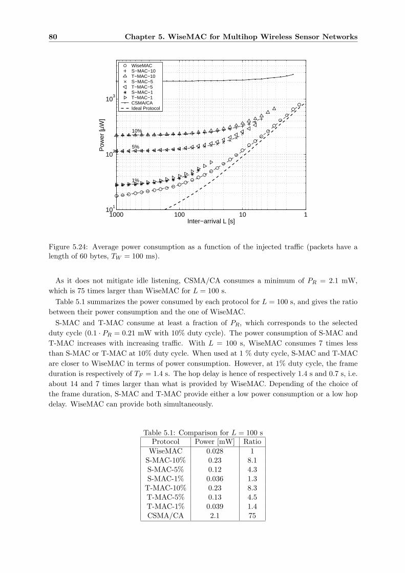
80 Chapter 5. WiseMAC for Multihop Wireless Sensor Networks
110100100010
1
102
103
10%
5%
1%
Pow
er [µ
W]
Inter−arrival L [s]
WiseMACS−MAC−10T−MAC−10S−MAC−5T−MAC−5S−MAC−1T−MAC−1CSMA/CAIdeal Protocol
Figure 5.24: Average power consumption as a function of the injected traffic (packets have alength of 60 bytes, TW = 100 ms).
As it does not mitigate idle listening, CSMA/CA consumes a minimum of PR = 2.1 mW,which is 75 times larger than WiseMAC for L = 100 s.
Table 5.1 summarizes the power consumed by each protocol for L = 100 s, and gives the ratiobetween their power consumption and the one of WiseMAC.
S-MAC and T-MAC consume at least a fraction of PR, which corresponds to the selectedduty cycle (0.1 · PR = 0.21 mW with 10% duty cycle). The power consumption of S-MAC andT-MAC increases with increasing traffic. With L = 100 s, WiseMAC consumes 7 times lessthan S-MAC or T-MAC at 10% duty cycle. When used at 1 % duty cycle, S-MAC and T-MACare closer to WiseMAC in terms of power consumption. However, at 1% duty cycle, the frameduration is respectively of TF = 1.4 s. The hop delay is hence of respectively 1.4 s and 0.7 s, i.e.about 14 and 7 times larger than what is provided by WiseMAC. Depending of the choice ofthe frame duration, S-MAC and T-MAC provide either a low power consumption or a low hopdelay. WiseMAC can provide both simultaneously.
Table 5.1: Comparison for L = 100 sProtocol Power [mW] Ratio
WiseMAC 0.028 1S-MAC-10% 0.23 8.1S-MAC-5% 0.12 4.3S-MAC-1% 0.036 1.3T-MAC-10% 0.23 8.3T-MAC-5% 0.13 4.5T-MAC-1% 0.039 1.4CSMA/CA 2.1 75
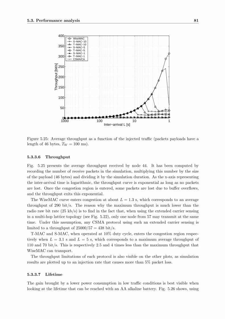
5.3. Performance analysis 81
11010010000
50
100
150
200
250
300
350
400
Thr
ough
put [
bit/s
]
Inter−arrival L [s]
WiseMACS−MAC−10T−MAC−10S−MAC−5T−MAC−5S−MAC−1T−MAC−1CSMA/CA
Figure 5.25: Average throughput as a function of the injected traffic (packets payloads have alength of 46 bytes, TW = 100 ms).
5.3.3.6 Throughput
Fig. 5.25 presents the average throughput received by node 44. It has been computed byrecording the number of receive packets in the simulation, multiplying this number by the sizeof the payload (46 bytes) and dividing it by the simulation duration. As the x-axis representingthe inter-arrival time is logarithmic, the throughput curve is exponential as long as no packetsare lost. Once the congestion region is entered, some packets are lost due to buffer overflows,and the throughput exits this exponential.
The WiseMAC curve enters congestion at about L = 1.3 s, which corresponds to an averagethroughput of 290 bit/s. The reason why the maximum throughput is much lower than theradio raw bit rate (25 kb/s) is to find in the fact that, when using the extended carrier sensingin a multi-hop lattice topology (see Fig. 5.22), only one node from 57 may transmit at the sametime. Under this assumption, any CSMA protocol using such an extended carrier sensing islimited to a throughput of 25000/57 = 438 bit/s.
T-MAC and S-MAC, when operated at 10% duty cycle, enters the congestion region respec-tively when L = 3.1 s and L = 5 s, which corresponds to a maximum average throughput of110 and 70 bit/s. This is respectively 2.5 and 4 times less than the maximum throughput thatWiseMAC can transport.
The throughput limitations of each protocol is also visible on the other plots, as simulationresults are plotted up to an injection rate that causes more than 5% packet loss.
5.3.3.7 Lifetime
The gain brought by a lower power consumption in low traffic conditions is best visible whenlooking at the lifetime that can be reached with an AA alkaline battery. Fig. 5.26 shows, using
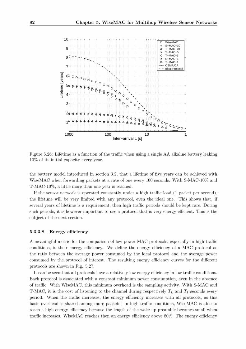
82 Chapter 5. WiseMAC for Multihop Wireless Sensor Networks
1101001000
1
2
3
4
5
6
7
8
9
10
Life
time
[yea
rs]
Inter−arrival L [s]
WiseMACS−MAC−10T−MAC−10S−MAC−5T−MAC−5S−MAC−1T−MAC−1CSMA/CAIdeal Protocol
Figure 5.26: Lifetime as a function of the traffic when using a single AA alkaline battery leaking10% of its initial capacity every year.
the battery model introduced in section 3.2, that a lifetime of five years can be achieved withWiseMAC when forwarding packets at a rate of one every 100 seconds. With S-MAC-10% andT-MAC-10%, a little more than one year is reached.
If the sensor network is operated constantly under a high traffic load (1 packet per second),the lifetime will be very limited with any protocol, even the ideal one. This shows that, ifseveral years of lifetime is a requirement, then high traffic periods should be kept rare. Duringsuch periods, it is however important to use a protocol that is very energy efficient. This is thesubject of the next section.
5.3.3.8 Energy efficiency
A meaningful metric for the comparison of low power MAC protocols, especially in high trafficconditions, is their energy efficiency. We define the energy efficiency of a MAC protocol asthe ratio between the average power consumed by the ideal protocol and the average powerconsumed by the protocol of interest. The resulting energy efficiency curves for the differentprotocols are shown in Fig. 5.27.
It can be seen that all protocols have a relatively low energy efficiency in low traffic conditions.Each protocol is associated with a constant minimum power consumption, even in the absenceof traffic. With WiseMAC, this minimum overhead is the sampling activity. With S-MAC andT-MAC, it is the cost of listening to the channel during respectively TL and TI seconds everyperiod. When the traffic increases, the energy efficiency increases with all protocols, as thisbasic overhead is shared among more packets. In high traffic conditions, WiseMAC is able toreach a high energy efficiency because the length of the wake-up preamble becomes small whentraffic increases. WiseMAC reaches then an energy efficiency above 80%. The energy efficiency
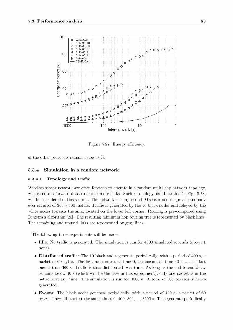
5.3. Performance analysis 83
11010010000
20
40
60
80
100
Ene
rgy
effic
ienc
y [%
]
Inter−arrival L [s]
WiseMACS−MAC−10T−MAC−10S−MAC−5T−MAC−5S−MAC−1T−MAC−1CSMA/CA
Figure 5.27: Energy efficiency.
of the other protocols remain below 50%.
5.3.4 Simulation in a random network
5.3.4.1 Topology and traffic
Wireless sensor network are often foreseen to operate in a random multi-hop network topology,where sensors forward data to one or more sinks. Such a topology, as illustrated in Fig. 5.28,will be considered in this section. The network is composed of 90 sensor nodes, spread randomlyover an area of 300× 300 meters. Traffic is generated by the 10 black nodes and relayed by thewhite nodes towards the sink, located on the lower left corner. Routing is pre-computed usingDijkstra’s algorithm [20]. The resulting minimum hop routing tree is represented by black lines.The remaining and unused links are represented by gray lines.
The following three experiments will be made:
• Idle: No traffic is generated. The simulation is run for 4000 simulated seconds (about 1hour).
• Distributed traffic: The 10 black nodes generate periodically, with a period of 400 s, apacket of 60 bytes. The first node starts at time 0, the second at time 40 s, ..., the lastone at time 360 s. Traffic is thus distributed over time. As long as the end-to-end delayremains below 40 s (which will be the case in this experiment), only one packet is in thenetwork at any time. The simulation is run for 4000 s. A total of 100 packets is hencegenerated.
• Events: The black nodes generate periodically, with a period of 400 s, a packet of 60bytes. They all start at the same times 0, 400, 800, ..., 3600 s. This generate periodically
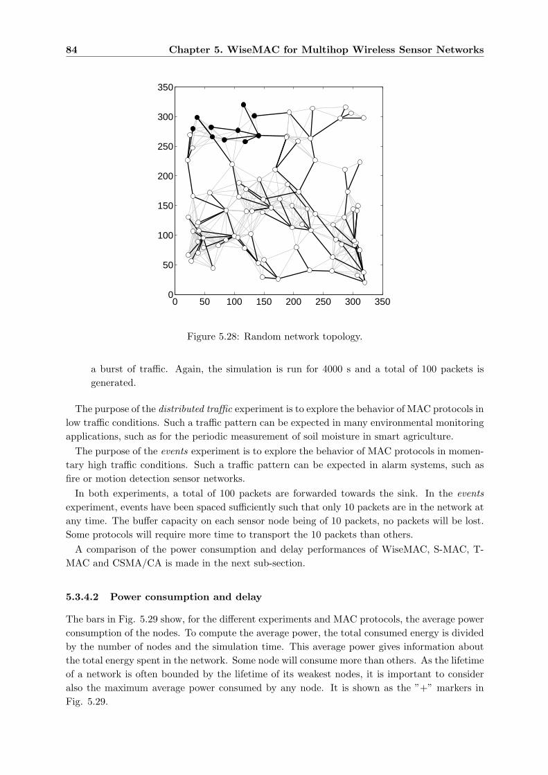
84 Chapter 5. WiseMAC for Multihop Wireless Sensor Networks
0 50 100 150 200 250 300 3500
50
100
150
200
250
300
350
Figure 5.28: Random network topology.
a burst of traffic. Again, the simulation is run for 4000 s and a total of 100 packets isgenerated.
The purpose of the distributed traffic experiment is to explore the behavior of MAC protocols inlow traffic conditions. Such a traffic pattern can be expected in many environmental monitoringapplications, such as for the periodic measurement of soil moisture in smart agriculture.
The purpose of the events experiment is to explore the behavior of MAC protocols in momen-tary high traffic conditions. Such a traffic pattern can be expected in alarm systems, such asfire or motion detection sensor networks.
In both experiments, a total of 100 packets are forwarded towards the sink. In the eventsexperiment, events have been spaced sufficiently such that only 10 packets are in the network atany time. The buffer capacity on each sensor node being of 10 packets, no packets will be lost.Some protocols will require more time to transport the 10 packets than others.
A comparison of the power consumption and delay performances of WiseMAC, S-MAC, T-MAC and CSMA/CA is made in the next sub-section.
5.3.4.2 Power consumption and delay
The bars in Fig. 5.29 show, for the different experiments and MAC protocols, the average powerconsumption of the nodes. To compute the average power, the total consumed energy is dividedby the number of nodes and the simulation time. This average power gives information aboutthe total energy spent in the network. Some node will consume more than others. As the lifetimeof a network is often bounded by the lifetime of its weakest nodes, it is important to consideralso the maximum average power consumed by any node. It is shown as the ”+” markers inFig. 5.29.
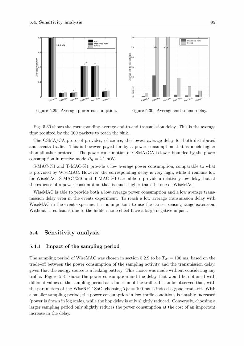
5.4. Sensitivity analysis 85
0
0.1
0.2
0.3
0.4A
vera
ge p
ower
[mW
]
CSMA/CASMAC1%
TMAC1%SMAC10%
TMAC10%WiseMAC
> 2.1 mW
IdleDistributed trafficEvents
Figure 5.29: Average power consumption.
012345
10
15
20
25
30
Ave
rage
end
−to
−en
d de
lay
[s]
CSMA/CASMAC1%
TMAC1%SMAC10%
TMAC10%WiseMAC
93 s 49 s
Distributed trafficEvents
Figure 5.30: Average end-to-end delay.
Fig. 5.30 shows the corresponding average end-to-end transmission delay. This is the averagetime required by the 100 packets to reach the sink.
The CSMA/CA protocol provides, of course, the lowest average delay for both distributedand events traffic. This is however payed for by a power consumption that is much higherthan all other protocols. The power consumption of CSMA/CA is lower bounded by the powerconsumption in receive mode PR = 2.1 mW.
S-MAC-%1 and T-MAC-%1 provide a low average power consumption, comparable to whatis provided by WiseMAC. However, the corresponding delay is very high, while it remains lowfor WiseMAC. S-MAC-%10 and T-MAC-%10 are able to provide a relatively low delay, but atthe expense of a power consumption that is much higher than the one of WiseMAC.
WiseMAC is able to provide both a low average power consumption and a low average trans-mission delay even in the events experiment. To reach a low average transmission delay withWiseMAC in the event experiment, it is important to use the carrier sensing range extension.Without it, collisions due to the hidden node effect have a large negative impact.
5.4 Sensitivity analysis
5.4.1 Impact of the sampling period
The sampling period of WiseMAC was chosen in section 5.2.9 to be TW = 100 ms, based on thetrade-off between the power consumption of the sampling activity and the transmission delay,given that the energy source is a leaking battery. This choice was made without considering anytraffic. Figure 5.31 shows the power consumption and the delay that would be obtained withdifferent values of the sampling period as a function of the traffic. It can be observed that, withthe parameters of the WiseNET SoC, choosing TW = 100 ms is indeed a good trade-off. Witha smaller sampling period, the power consumption in low traffic conditions is notably increased(power is drawn in log scale), while the hop delay is only slightly reduced. Conversely, choosing alarger sampling period only slightly reduces the power consumption at the cost of an importantincrease in the delay.
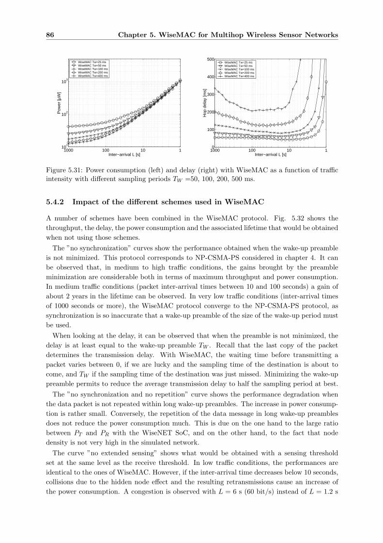
86 Chapter 5. WiseMAC for Multihop Wireless Sensor Networks
110100100010
1
102
103
Pow
er [µ
W]
Inter−arrival L [s]
WiseMAC Tw=25 msWiseMAC Tw=50 msWiseMAC Tw=100 msWiseMAC Tw=200 msWiseMAC Tw=400 ms
11010010000
100
200
300
400
500
Hop
del
ay [m
s]
Inter−arrival L [s]
WiseMAC Tw=25 msWiseMAC Tw=50 msWiseMAC Tw=100 msWiseMAC Tw=200 msWiseMAC Tw=400 ms
Figure 5.31: Power consumption (left) and delay (right) with WiseMAC as a function of trafficintensity with different sampling periods TW =50, 100, 200, 500 ms.
5.4.2 Impact of the different schemes used in WiseMAC
A number of schemes have been combined in the WiseMAC protocol. Fig. 5.32 shows thethroughput, the delay, the power consumption and the associated lifetime that would be obtainedwhen not using those schemes.
The ”no synchronization” curves show the performance obtained when the wake-up preambleis not minimized. This protocol corresponds to NP-CSMA-PS considered in chapter 4. It canbe observed that, in medium to high traffic conditions, the gains brought by the preambleminimization are considerable both in terms of maximum throughput and power consumption.In medium traffic conditions (packet inter-arrival times between 10 and 100 seconds) a gain ofabout 2 years in the lifetime can be observed. In very low traffic conditions (inter-arrival timesof 1000 seconds or more), the WiseMAC protocol converge to the NP-CSMA-PS protocol, assynchronization is so inaccurate that a wake-up preamble of the size of the wake-up period mustbe used.
When looking at the delay, it can be observed that when the preamble is not minimized, thedelay is at least equal to the wake-up preamble TW . Recall that the last copy of the packetdetermines the transmission delay. With WiseMAC, the waiting time before transmitting apacket varies between 0, if we are lucky and the sampling time of the destination is about tocome, and TW if the sampling time of the destination was just missed. Minimizing the wake-uppreamble permits to reduce the average transmission delay to half the sampling period at best.
The ”no synchronization and no repetition” curve shows the performance degradation whenthe data packet is not repeated within long wake-up preambles. The increase in power consump-tion is rather small. Conversely, the repetition of the data message in long wake-up preamblesdoes not reduce the power consumption much. This is due on the one hand to the large ratiobetween PT and PR with the WiseNET SoC, and on the other hand, to the fact that nodedensity is not very high in the simulated network.
The curve ”no extended sensing” shows what would be obtained with a sensing thresholdset at the same level as the receive threshold. In low traffic conditions, the performances areidentical to the ones of WiseMAC. However, if the inter-arrival time decreases below 10 seconds,collisions due to the hidden node effect and the resulting retransmissions cause an increase ofthe power consumption. A congestion is observed with L = 6 s (60 bit/s) instead of L = 1.2 s
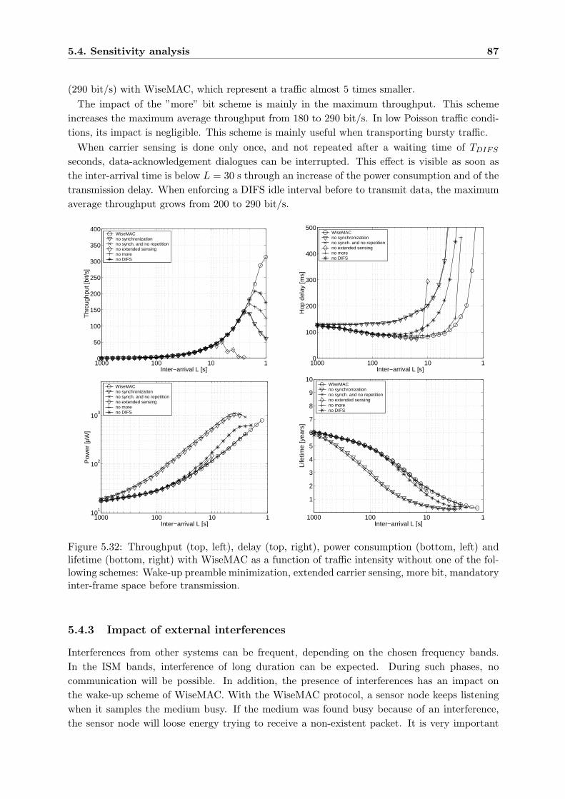
5.4. Sensitivity analysis 87
(290 bit/s) with WiseMAC, which represent a traffic almost 5 times smaller.The impact of the ”more” bit scheme is mainly in the maximum throughput. This scheme
increases the maximum average throughput from 180 to 290 bit/s. In low Poisson traffic condi-tions, its impact is negligible. This scheme is mainly useful when transporting bursty traffic.
When carrier sensing is done only once, and not repeated after a waiting time of TDIFS
seconds, data-acknowledgement dialogues can be interrupted. This effect is visible as soon asthe inter-arrival time is below L = 30 s through an increase of the power consumption and of thetransmission delay. When enforcing a DIFS idle interval before to transmit data, the maximumaverage throughput grows from 200 to 290 bit/s.
11010010000
50
100
150
200
250
300
350
400
Thr
ough
put [
bit/s
]
Inter−arrival L [s]
WiseMACno synchronizationno synch. and no repetitionno extended sensingno moreno DIFS
11010010000
100
200
300
400
500
Hop
del
ay [m
s]
Inter−arrival L [s]
WiseMACno synchronizationno synch. and no repetitionno extended sensingno moreno DIFS
110100100010
1
102
103
Pow
er [µ
W]
Inter−arrival L [s]
WiseMACno synchronizationno synch. and no repetitionno extended sensingno moreno DIFS
1101001000
1
2
3
4
5
6
7
8
9
10
Life
time
[yea
rs]
Inter−arrival L [s]
WiseMACno synchronizationno synch. and no repetitionno extended sensingno moreno DIFS
Figure 5.32: Throughput (top, left), delay (top, right), power consumption (bottom, left) andlifetime (bottom, right) with WiseMAC as a function of traffic intensity without one of the fol-lowing schemes: Wake-up preamble minimization, extended carrier sensing, more bit, mandatoryinter-frame space before transmission.
5.4.3 Impact of external interferences
Interferences from other systems can be frequent, depending on the chosen frequency bands.In the ISM bands, interference of long duration can be expected. During such phases, nocommunication will be possible. In addition, the presence of interferences has an impact onthe wake-up scheme of WiseMAC. With the WiseMAC protocol, a sensor node keeps listeningwhen it samples the medium busy. If the medium was found busy because of an interference,the sensor node will loose energy trying to receive a non-existent packet. It is very important
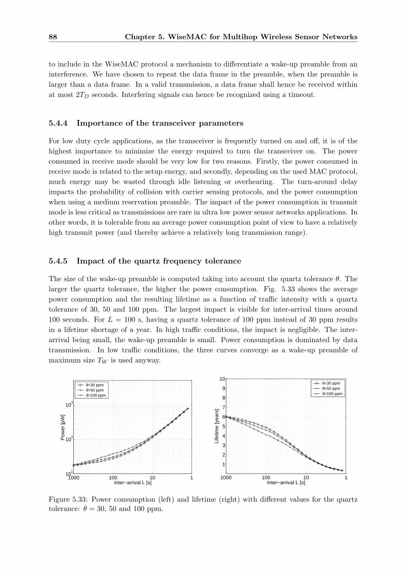
88 Chapter 5. WiseMAC for Multihop Wireless Sensor Networks
to include in the WiseMAC protocol a mechanism to differentiate a wake-up preamble from aninterference. We have chosen to repeat the data frame in the preamble, when the preamble islarger than a data frame. In a valid transmission, a data frame shall hence be received withinat most 2TD seconds. Interfering signals can hence be recognized using a timeout.
5.4.4 Importance of the transceiver parameters
For low duty cycle applications, as the transceiver is frequently turned on and off, it is of thehighest importance to minimize the energy required to turn the transceiver on. The powerconsumed in receive mode should be very low for two reasons. Firstly, the power consumed inreceive mode is related to the setup energy, and secondly, depending on the used MAC protocol,much energy may be wasted through idle listening or overhearing. The turn-around delayimpacts the probability of collision with carrier sensing protocols, and the power consumptionwhen using a medium reservation preamble. The impact of the power consumption in transmitmode is less critical as transmissions are rare in ultra low power sensor networks applications. Inother words, it is tolerable from an average power consumption point of view to have a relativelyhigh transmit power (and thereby achieve a relatively long transmission range).
5.4.5 Impact of the quartz frequency tolerance
The size of the wake-up preamble is computed taking into account the quartz tolerance θ. Thelarger the quartz tolerance, the higher the power consumption. Fig. 5.33 shows the averagepower consumption and the resulting lifetime as a function of traffic intensity with a quartztolerance of 30, 50 and 100 ppm. The largest impact is visible for inter-arrival times around100 seconds. For L = 100 s, having a quartz tolerance of 100 ppm instead of 30 ppm resultsin a lifetime shortage of a year. In high traffic conditions, the impact is negligible. The inter-arrival being small, the wake-up preamble is small. Power consumption is dominated by datatransmission. In low traffic conditions, the three curves converge as a wake-up preamble ofmaximum size TW is used anyway.
110100100010
1
102
103
Pow
er [µ
W]
Inter−arrival L [s]
θ=30 ppmθ=50 ppmθ=100 ppm
1101001000
1
2
3
4
5
6
7
8
9
10
Life
time
[yea
rs]
Inter−arrival L [s]
θ=30 ppmθ=50 ppmθ=100 ppm
Figure 5.33: Power consumption (left) and lifetime (right) with different values for the quartztolerance: θ = 30, 50 and 100 ppm.
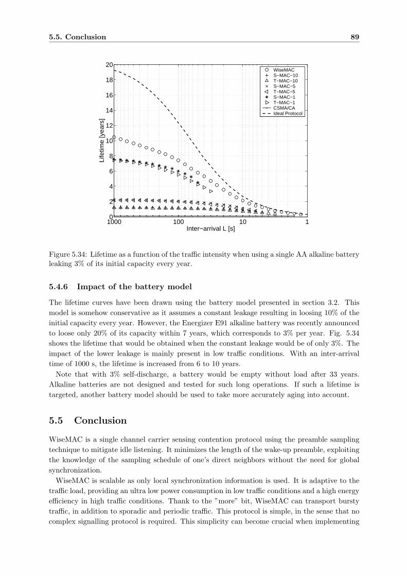
5.5. Conclusion 89
11010010000
2
4
6
8
10
12
14
16
18
20
Life
time
[yea
rs]
Inter−arrival L [s]
WiseMACS−MAC−10T−MAC−10S−MAC−5T−MAC−5S−MAC−1T−MAC−1CSMA/CAIdeal Protocol
Figure 5.34: Lifetime as a function of the traffic intensity when using a single AA alkaline batteryleaking 3% of its initial capacity every year.
5.4.6 Impact of the battery model
The lifetime curves have been drawn using the battery model presented in section 3.2. Thismodel is somehow conservative as it assumes a constant leakage resulting in loosing 10% of theinitial capacity every year. However, the Energizer E91 alkaline battery was recently announcedto loose only 20% of its capacity within 7 years, which corresponds to 3% per year. Fig. 5.34shows the lifetime that would be obtained when the constant leakage would be of only 3%. Theimpact of the lower leakage is mainly present in low traffic conditions. With an inter-arrivaltime of 1000 s, the lifetime is increased from 6 to 10 years.
Note that with 3% self-discharge, a battery would be empty without load after 33 years.Alkaline batteries are not designed and tested for such long operations. If such a lifetime istargeted, another battery model should be used to take more accurately aging into account.
5.5 Conclusion
WiseMAC is a single channel carrier sensing contention protocol using the preamble samplingtechnique to mitigate idle listening. It minimizes the length of the wake-up preamble, exploitingthe knowledge of the sampling schedule of one’s direct neighbors without the need for globalsynchronization.
WiseMAC is scalable as only local synchronization information is used. It is adaptive to thetraffic load, providing an ultra low power consumption in low traffic conditions and a high energyefficiency in high traffic conditions. Thank to the ”more” bit, WiseMAC can transport burstytraffic, in addition to sporadic and periodic traffic. This protocol is simple, in the sense that nocomplex signalling protocol is required. This simplicity can become crucial when implementing
90 Chapter 5. WiseMAC for Multihop Wireless Sensor Networks
it on devices with very limited computational resources.WiseMAC was compared to S-MAC and T-MAC both in a regular lattice topology with
traffic flowing in parallel, and in a random network topology with periodic or event trafficflowing towards a sink. When forwarding packets at an interval of 1 packets every 100 seconds,the power consumption of WiseMAC was found to be 28 µW, providing 5 years of lifetimeusing a single AA alkaline battery. This is 75 times better than CSMA/CA and 8 times betterthan S-MAC and T-MAC at a duty cycle of 10%. It was shown that WiseMAC can providesimultaneously a low hop delay and a low power consumption, while S-MAC and T-MAC canonly provide one or the other. Finally, it was shown that WiseMAC is able to transport a highertraffic intensity than both S-MAC-10% and T-MAC-10%.
Chapter 6
Downlink of an Infrastructure
Wireless Sensor Network
6.1 Introduction
6.1.1 Problem statement
An infrastructure wireless network is composed of a number of access points interconnectedthrough a backbone network. Each access point is serving a number of wireless sensor nodes.Such a topology, illustrated in Fig. 6.1, can be envisaged for example in smart building ap-plications, where the Ethernet or powerline cabling can be used as a backbone network. Themain characteristic of access points is that they are usually energy unconstrained. This fact canbe exploited by medium access control protocols in two ways: first, an access point can listencontinuously to potential uplink traffic, and secondly, an access point may send any amount ofsignalling traffic for free (e.g. beacons, wake-up signal). The WiseMAC protocol was designedfor multi-hop networks. The work presented in this chapter was initiated to verify whetherWiseMAC should also be used for the communication between an access point and a sensornode, or whether other protocols should be preferred. This work also applies to other systemswhere energy unconstrained nodes can play the role of base stations, such as clustered ad-hocnetworks with solar powered cluster heads [69] or vehicle mounted mobile access points movingthrough a cloud of sensors to collect data.
In infrastructure networks, one must distinguish the downlink (from the access point to thesensor nodes) from the uplink (from the sensor nodes to the access point). For each direction,a different radio frequency and/or a different MAC protocol may be used.
In the downlink direction, the challenge is to transmit data from the access point to somesensor node, without requiring that the sensor node continuously listen to the channel. A trade-off must be made between power consumption and transmission delay.
The problem is different in the uplink direction. As the access point is not energy limited, itcan listen all the time to the channel. The issue to resolve in the uplink is the multiple access toa shared medium. If the system is operated near channel capacity, this problem is very complex.However, if only moderate traffic is present on the channel, finding a energy efficient uplinkMAC protocol is relatively easy. For example, the simple non-persistent CSMA protocol [58]approaches the ideal case for power conservation, with no idle listening, no overhearing and littlecollisions.
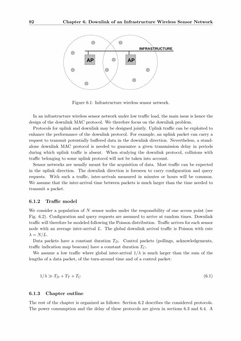
92 Chapter 6. Downlink of an Infrastructure Wireless Sensor Network
INFRASTRUCTURE
AP AP
Figure 6.1: Infrastructure wireless sensor network.
In an infrastructure wireless sensor network under low traffic load, the main issue is hence thedesign of the downlink MAC protocol. We therefore focus on the downlink problem.
Protocols for uplink and downlink may be designed jointly. Uplink traffic can be exploited toenhance the performance of the downlink protocol. For example, an uplink packet can carry arequest to transmit potentially buffered data in the downlink direction. Nevertheless, a stand-alone downlink MAC protocol is needed to guarantee a given transmission delay in periodsduring which uplink traffic is absent. When studying the downlink protocol, collisions withtraffic belonging to some uplink protocol will not be taken into account.
Sensor networks are usually meant for the acquisition of data. Most traffic can be expectedin the uplink direction. The downlink direction is foreseen to carry configuration and queryrequests. With such a traffic, inter-arrivals measured in minutes or hours will be common.We assume that the inter-arrival time between packets is much larger than the time needed totransmit a packet.
6.1.2 Traffic model
We consider a population of N sensor nodes under the responsibility of one access point (seeFig. 6.2). Configuration and query requests are assumed to arrive at random times. Downlinktraffic will therefore be modeled following the Poisson distribution. Traffic arrives for each sensornode with an average inter-arrival L. The global downlink arrival traffic is Poisson with rateλ = N/L.
Data packets have a constant duration TD. Control packets (pollings, acknowledgements,traffic indication map beacons) have a constant duration TC .
We assume a low traffic where global inter-arrival 1/λ is much larger than the sum of thelengths of a data packet, of the turn-around time and of a control packet:
1/λ À TD + TT + TC (6.1)
6.1.3 Chapter outline
The rest of the chapter is organized as follows: Section 6.2 describes the considered protocols.The power consumption and the delay of these protocols are given in sections 6.3 and 6.4. A
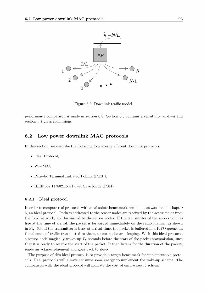
6.2. Low power downlink MAC protocols 93
AP
1
2
3
N-1
N
=N/L
1/L
Figure 6.2: Downlink traffic model.
performance comparison is made in section 6.5. Section 6.6 contains a sensitivity analysis andsection 6.7 gives conclusions.
6.2 Low power downlink MAC protocols
In this section, we describe the following four energy efficient downlink protocols:
• Ideal Protocol,
• WiseMAC,
• Periodic Terminal Initiated Polling (PTIP),
• IEEE 802.11/802.15.4 Power Save Mode (PSM)
6.2.1 Ideal protocol
In order to compare real protocols with an absolute benchmark, we define, as was done in chapter5, an ideal protocol. Packets addressed to the sensor nodes are received by the access point fromthe fixed network, and forwarded to the sensor nodes. If the transmitter of the access point isfree at the time of arrival, the packet is forwarded immediately on the radio channel, as shownin Fig. 6.3. If the transmitter is busy at arrival time, the packet is buffered in a FIFO queue. Inthe absence of traffic transmitted to them, sensor nodes are sleeping. With this ideal protocol,a sensor node magically wakes up TS seconds before the start of the packet transmission, suchthat it is ready to receive the start of the packet. It then listens for the duration of the packet,sends an acknowledgement and goes back to sleep.
The purpose of this ideal protocol is to provide a target benchmark for implementable proto-cols. Real protocols will always consume some energy to implement the wake-up scheme. Thecomparison with the ideal protocol will indicate the cost of each wake-up scheme.
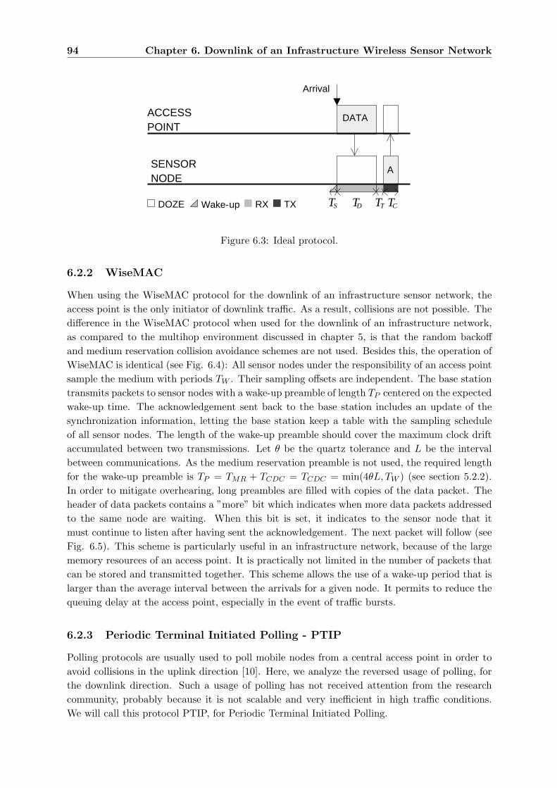
94 Chapter 6. Downlink of an Infrastructure Wireless Sensor Network
ACCESSPOINT
SENSORNODE
A
Arrival
DATA
TD TCTTTSDOZE RX TXWake-up
Figure 6.3: Ideal protocol.
6.2.2 WiseMAC
When using the WiseMAC protocol for the downlink of an infrastructure sensor network, theaccess point is the only initiator of downlink traffic. As a result, collisions are not possible. Thedifference in the WiseMAC protocol when used for the downlink of an infrastructure network,as compared to the multihop environment discussed in chapter 5, is that the random backoffand medium reservation collision avoidance schemes are not used. Besides this, the operation ofWiseMAC is identical (see Fig. 6.4): All sensor nodes under the responsibility of an access pointsample the medium with periods TW . Their sampling offsets are independent. The base stationtransmits packets to sensor nodes with a wake-up preamble of length TP centered on the expectedwake-up time. The acknowledgement sent back to the base station includes an update of thesynchronization information, letting the base station keep a table with the sampling scheduleof all sensor nodes. The length of the wake-up preamble should cover the maximum clock driftaccumulated between two transmissions. Let θ be the quartz tolerance and L be the intervalbetween communications. As the medium reservation preamble is not used, the required lengthfor the wake-up preamble is TP = TMR + TCDC = TCDC = min(4θL, TW ) (see section 5.2.2).In order to mitigate overhearing, long preambles are filled with copies of the data packet. Theheader of data packets contains a ”more” bit which indicates when more data packets addressedto the same node are waiting. When this bit is set, it indicates to the sensor node that itmust continue to listen after having sent the acknowledgement. The next packet will follow (seeFig. 6.5). This scheme is particularly useful in an infrastructure network, because of the largememory resources of an access point. It is practically not limited in the number of packets thatcan be stored and transmitted together. This scheme allows the use of a wake-up period that islarger than the average interval between the arrivals for a given node. It permits to reduce thequeuing delay at the access point, especially in the event of traffic bursts.
6.2.3 Periodic Terminal Initiated Polling - PTIP
Polling protocols are usually used to poll mobile nodes from a central access point in order toavoid collisions in the uplink direction [10]. Here, we analyze the reversed usage of polling, forthe downlink direction. Such a usage of polling has not received attention from the researchcommunity, probably because it is not scalable and very inefficient in high traffic conditions.We will call this protocol PTIP, for Periodic Terminal Initiated Polling.
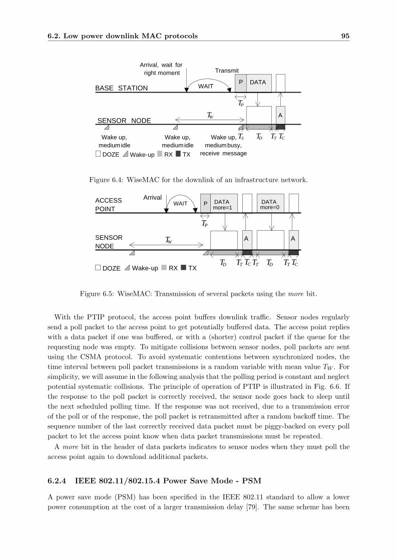
6.2. Low power downlink MAC protocols 95
BASE STATION
SENSOR NODEA
WAIT
Arrival, wait forright moment
P DATA
Transmit
Wake up,mediumidle
Wake up,mediumidle
Wake up, mediumbusy,
receive message
TW
DOZE RX TXWake-up
TD TCTTTS
TP
Figure 6.4: WiseMAC for the downlink of an infrastructure network.
ACCESSPOINT
SENSORNODE
WAITArrival
TWA
DATA
A
P DATAmore=1 more=0
Wake-upDOZE RX TXTD TCTT
TP
TT TTTDTC
Figure 6.5: WiseMAC: Transmission of several packets using the more bit.
With the PTIP protocol, the access point buffers downlink traffic. Sensor nodes regularlysend a poll packet to the access point to get potentially buffered data. The access point replieswith a data packet if one was buffered, or with a (shorter) control packet if the queue for therequesting node was empty. To mitigate collisions between sensor nodes, poll packets are sentusing the CSMA protocol. To avoid systematic contentions between synchronized nodes, thetime interval between poll packet transmissions is a random variable with mean value TW . Forsimplicity, we will assume in the following analysis that the polling period is constant and neglectpotential systematic collisions. The principle of operation of PTIP is illustrated in Fig. 6.6. Ifthe response to the poll packet is correctly received, the sensor node goes back to sleep untilthe next scheduled polling time. If the response was not received, due to a transmission errorof the poll or of the response, the poll packet is retransmitted after a random backoff time. Thesequence number of the last correctly received data packet must be piggy-backed on every pollpacket to let the access point know when data packet transmissions must be repeated.
A more bit in the header of data packets indicates to sensor nodes when they must poll theaccess point again to download additional packets.
6.2.4 IEEE 802.11/802.15.4 Power Save Mode - PSM
A power save mode (PSM) has been specified in the IEEE 802.11 standard to allow a lowerpower consumption at the cost of a larger transmission delay [79]. The same scheme has been

96 Chapter 6. Downlink of an Infrastructure Wireless Sensor Network
POLL
ACCESSPOINT
SENSORNODE
POLL
DATANO
DATA
TW
TC TT TD
Arrival
TS
DOZE RX TXWake-up
TCTTTS TC
Figure 6.6: Periodic Terminal Initiated Polling (PTIP).
selected for the newer IEEE 802.15.4 standard [82]. The access point buffers incoming traffic. Abeacon is periodically transmitted with period TW . This beacon contains the traffic indicationmap (TIM), which lists the sensor nodes for which data packets have been buffered. All sensornodes wake up regularly to receive the TIM. If a sensor node finds its address in the TIM,its sends a poll packet to the access point, demanding the transmission of the announced datapacket.
The standard requires the access point to reply to a poll packet after a given delay (10 µs
in DSSS IEEE 802.11b). In practice, it is difficult for the access point software to find theright packet and prepare it for transmission within the specified delay. Instead, the accesspoint replies to the poll packet with an acknowledgement packet. This instructs the sensornode to remain in listening mode. As soon as possible, the access point sends the data packet,which is then acknowledged back by the sensor node. In summary, the polling procedure iscomposed of four packet transmissions: POLL-ACK-DATA-ACK. We are interested here in thebasic performance of protocols that would use a traffic indication map. For a fair comparisonwith the other protocols, we consider a version of the PSM protocol that is fully optimized forlow power operation. We assume first that an access point replies to a poll packet with a datapacket and secondly that a data packet is not acknowledged (as in PTIP, the acknowledgementis piggy-backed on the following poll packet). This procedure is illustrated in Fig. 6.7.
A more bit in the header of data packets indicates to sensor nodes when they must poll theaccess point again to download the additional packets.
In Fig. 6.7, the periods during which a sensor node is receiving are marked with a light graybar below the time line. The periods during which a sensor node is transmitting are markedwith a dark gray bar. One can observe that the sensor node starts listening TSync secondsbefore the actual start of the TIM packet. This behavior is required to compensate for theclock drift between the quartz running on the access point and on a sensor node. It was shownin the equivalent case of TDMA (chapter 4, section 4.2.2), that the duration of the requiredsynchronization period is TSync = 4θTW in the worst case. Taking the average over the possiblequartz inaccuracies, assuming a uniform distribution of the quartz inaccuracies, we have
TSync = 2θTW (6.2)
A sensor node may learn the relative difference between the frequency of its clock and ofthe clock running on the access point, and reduce the required synchronization time TSync.

6.3. Power consumption 97
ArrivalACCESSPOINT
SENSORNODE
TIM
POLL
TIM DATA
TSync
TW
TCTC TT TT TDTSDOZE RX TXWake-up
Figure 6.7: Optimized Power Save Mode (PSM).
This optimization has not been considered here. It will be seen later, that even without thisoptimization, the average power required for periodic re-synchronization is very small.
6.2.5 Adaptability of the wake-up period
Different nodes may have different delay requirements. For example, a light switch must reactto a command within less than a second, while a meter reader could answer to an automateddata collecting center within minutes. It is important for a MAC protocol to allow differentnodes to use different wake-up periods within the same network. This feature is available withall three protocols:
• With WiseMAC, the access point has to remember the sampling period of each sensornode, and compute the wake-up preamble length accordingly,
• With PTIP, each node is free to choose its polling period. The access point doesn’t evenhave to know them,
• With PSM, a node may decide to listen to each TIM broadcast. It may also choose to skipsome of them. The data frames will remain buffered as long as they have not been polled.The wake-up period can hence be freely chosen as a multiple of the TIM broadcast period.
6.3 Power consumption
In this section, we derive analytical expressions for the power consumption of the four protocols:Ideal, WiseMAC, PTIP and PSM. This analysis brings an insight into the sources of energywaste of these protocols, and allows their comparison.
6.3.1 Power consumption of the ideal protocol
We start the analysis with the easiest case: the ideal protocol. Packets received from thefixed network are queued and transmitted in FIFO order on the radio channel. Sensor nodes”magically” wake up just at the right time to receive the packets addressed to them. Packetsare acknowledged by the sensor nodes.
A sensor node receives one packet of length TD every L seconds on average. The energeticincrement cost of receiving one packet is EIDEAL = PSTS + PR(TD + TT ) + PT TC . This is theincrement compared to what would have been consumed when being in the doze state. In this
98 Chapter 6. Downlink of an Infrastructure Wireless Sensor Network
sum, PSTS is the energy required to power-on the transceiver into receive mode. PRTD is theenergy to receive the packet. PRTT is the energy to turn-around the transceiver into transmitmode and PT TC is the energy to send the acknowledgement. On average, we obtain a powerconsumption of
PIDEAL = PZ +PSTS + PR(TD + TT ) + PT TC
L(6.3)
In this expression, it is important not to neglect the setup and turn-around phases, as theenergy consumed in these states can exceed the energy consumed to receive the data packet.Indeed, with a high transmission rate, the energy PRTD needed to receive a packet of a few tensof bytes may be smaller than the setup energy PSTS .
6.3.2 Power consumption of WiseMAC
The power consumption of a sensor node using the WiseMAC protocol and receiving packetswith an average inter-arrival L is given by
PWiseMAC = PZ +PSTS + PRTI
TW
+PR(TLP + TD + TT ) + PT TC
L
+ PR(N − 1)TO
L
(6.4)
where the first term accounts for the power consumption in doze state, the second termaccounts for the increment caused by the sampling activity, the third term the increment causedby the reception and acknowledgement, and the last term the overhearing of the transmissionto the N − 1 other nodes. TLP is the average duration during which a sensor node that is thedestination of a message listens to the wake-up preamble. TO is the average duration duringwhich a node overhearers a transmission. As introduced in chapter 5, expressions (5.21) and(5.22), we have
TLP = 2θL(1− e−
TD4θL
)
and
TO =T 2
D + 12TDθL
2TW
(1− e−
TW4θL
)
Expression (6.4) is very similar to the power consumption in the multi-hop case (5.19). Thedifference is that transmission power consumption is not taken into account.
6.3.3 Power consumption of PTIP
Assuming no collisions between poll packets, the average power consumed by PTIP to receivedata packets with an average inter-arrival L is given by
6.3. Power consumption 99
PPTIP = PZ + e−TWL
PSTS + PT TC + PR(TT + TC)TW
+PSTS + PT TC + PR(TT + TD)
L
(6.5)
The fist term is the power consumed in doze mode. The second term accounts for uselesspolling, i.e. polling done when no data packet was waiting. The third term accounts for thepolling of buffered data packets.
To derive expression (6.5), let us first compute the energy spent in a period TW . With PTIP,as said previously, a sensor node sends a poll packet every TW seconds to the access point. Datapackets addressed to this sensor node arrive at the access point following a Poisson process of rate1/L. With probability e−
1L , no data packet will be waiting for this node. The access point will
reply with a short control packet. This event will consume an energy PSTS+PT TC+PRTT +PRTC
(setup, send the poll, turn around, receive the control packet). With probability 1− e−1L , k ≥ 1
data packets will be waiting in the buffer. In cases where k > 1 data packets are buffered, theyare all downloaded in a row thanks to the more bit which indicates when further data packetsare waiting. Let K1 be the average number of buffered data packets, given that at least one datapacket is present. The sensor node will consume an energy K1
(PSTS + PT TC + PR(TT + TD)
)
to download all data packets1. The average energy consumed by PTIP to receive the datapackets that have been buffered at the access point in a period TW is hence given by
EPTIP = e−TWL
(PSTS + PT TC + PR(TT + TC)
)
+ (1− e−TWL )K1
(PSTS + PT TC + PR(TT + TD)
) (6.6)
K1 can be computed as follows: With a Poisson arrival of rate 1/L, the average number ofarrivals in a period TW is K = TW
L . Here, we are interested in the average number of arrivals,
given that we have at least one arrival. There will be zero arrivals with probability e−TWL and
at least one arrival with probability 1− e−TWL . We know that K = e−
TWL · 0 +
(1− e−
TWL
)·K1.
Hence,
K1 =TWL
1− e−TWL
(6.7)
Combining (6.7) with (6.6), dividing by TW , adding PZ , one obtains (6.5).In this analysis, we have neglected the power consumption of retransmissions. As poll packets
are sent using the CSMA protocol, there is a risk to see poll packets sent by different sensornodes collide. Expression (6.5) is hence accurate only for large polling periods and low downlinktraffic conditions. This point will be addressed in more details when looking at the transmissiondelay.
1If several data packets are downloaded in a row, the transceiver will need an energy PSTS to turn thetransceiver on before sending the first poll packet. A smaller energy PRTT will be needed before to send thesubsequent poll packets. To be accurate, one must hence consider that expression (6.5) is an upper bound on thepower consumption of PTIP.
100 Chapter 6. Downlink of an Infrastructure Wireless Sensor Network
6.3.4 Power consumption of PSM
Under the assumptions that a poll packet is directly answered with a data packet, and that adata packet is acknowledged in the subsequent poll, the average power consumed by PSM toreceive packets with an average inter-arrival L is given by
PPSM = PZ + 2θPR +PSTS + PRTC
TW+
PT TC + PR(TD + 2TT )L
(6.8)
The first term represents the power consumed in doze mode. The second term, 2θPR, accountsfor the time spent listening to the channel to cover the drift between the access point clock andthe sensor node clock. The third term represents the power consumed to power-on and listen tothe beacon of length TC every TW seconds. Finally, the fourth term accounts for the receptionand acknowledgement of data packets.
To derive expression (6.8), let us first compute the energy spent in a period TW . We assumethat all traffic arriving during a period TW is polled during the following period TW . We donot consider bursty arrivals that require several periods to be downloaded. Multiple arrivalsfor a single sensor node are detected by the sensor node thanks to the more bit. Under theseassumptions, the energy spent by a sensor node in a period TW is composed of the energy toreceive the beacon PSTS + PR(TSync +TC) and the energy to download all TW
L buffered packets.We have
EPSM = PSTS + PR(TSync + TC) +TW
L
(PT TC + PR(TD + 2TT )
)(6.9)
PSTS + PR(TSync + TC) represents the energy to power-on the transceiver, to listen to themedium until the beacon transmission starts and to listen to the beacon. PT TC + PR(TD +2TT )represents the energy to send the poll packet and receive the data. Here, we count also theturn-around phases before sending the poll and before receiving the data. Combining (6.9) with(6.2), dividing by TW , adding PZ , one obtains (6.8).
As in the case of PTIP, we have neglected the impact of retransmissions of poll packetsrequired in case of collisions. This point will also be addressed in more details when looking atthe transmission delay.
6.4 Transmission delay
The transmission delay is defined as the time elapsed between the arrival of a packet at theaccess point and the end of its reception by the destination sensor node. In this section, usingan approximation analysis, we derive the transmission delay obtained using the four protocolsunder investigation.
6.4.1 Delay with the ideal protocol
In the case of the ideal protocol, packets of fixed length TD arrive following a Poisson processof rate λ. They are buffered in a FIFO buffer and transmitted sequentially. The average delay
6.4. Transmission delay 101
of this M/D/1 queue is given by
DIDEAL = TD +λm2
2(1− λm)
where m = TD +TT +TC +TT (see [8]). As 1/λ À TD +TT +TC (low traffic assumption (6.1)),we have
DIDEAL ≈ TD (6.10)
6.4.2 Delay with WiseMAC
To compute the average delay with WiseMAC, we will consider that the access point has oneFIFO queue for each sensor node. Incoming packets are stored in the FIFO queue of therespective destination. Following some policy, the access point chooses a queue to serve. Thanksto the more bit, all packets are sent to the chosen sensor node in a row, starting at the instantwhen this sensor node samples the medium. To avoid having a large number of packets in thequeues, one must choose a policy that maximizes the channel utilization. Once a queue has beenserved, such a policy is to choose, as the next queue to be served, the one of the sensor nodewhich is next going to sample the medium. Based on this policy, and as 1/λ À TD+TT +TC (lowtraffic assumption (6.1)), we can assume that every queue is served after at most TW seconds.
We will start by computing the transmission delay considering that a single packet is senttowards a given sensor node, i.e. only one packet destined to this node has arrived at the basestation in the period of duration TW preceding the transmission. We will next see that theaverage time needed to transmit possible additional packets is negligible.
A data packet is transmitted with a preamble of length TP = min(4θl, TW ). Depending onthe value of the interval l between two communications with a given node, the three followingscenarios are possible (see also Fig. 5.11):
A) TP < TD,
B) TW > TP ≥ TD,
C) TP = TW .
In scenario A, the packet must first wait for the right transmission time. The duration of thewait time can vary between 0 (if this packet is lucky) and TW . On average, the wait time isequal to TW
2 . Then, one must count the time to transmit the wake-up preamble and the data.We have DA = TW
2 + 4θl + TD.Scenario B is different from scenario A because the wake-up preamble is composed of copies
of the data frame. The first delay is again the waiting delay TW2 . During the transmission of the
wake-up preamble, the destination node may wake up at any instant. On average, it will wakeup after TP
2 = 2θl seconds. Once awake, the node waits for the start of the next copy of the datapacket (TD
2 on average) and then receives the data packet. We have DB = TW2 + 2θl + TD
2 + TD.In scenario C, the synchronization is assumed to be lost. The wake-up preamble has the length
of the sampling period. The transmission is started as soon as the packet is received by the basestation. The destination will, on average, sample the medium after TW
2 seconds of preamble
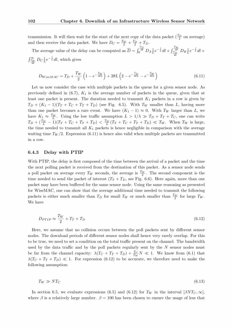
102 Chapter 6. Downlink of an Infrastructure Wireless Sensor Network
transmission. It will then wait for the start of the next copy of the data packet (TD2 on average)
and then receive the data packet. We have DC = TW2 + TD
2 + TD.
The average value of the delay can be computed as D =∫ TD
4θ0 DA
1Le−
lL dl +
∫ TW4θ
TD4θ
DB1Le−
lL dl +
∫∞TW4θ
DC1Le−
lL dl, which gives
DWiseMAC = TD +TW
2
(1− e−
TW4θL
)+ 2θL
(2− e−
TD4θL − e−
TW4θL
)(6.11)
Let us now consider the case with multiple packets in the queue for a given sensor node. Aspreviously defined in (6.7), K1 is the average number of packets in the queue, given that atleast one packet is present. The duration needed to transmit K1 packets in a row is given byTD + (K1 − 1)(TT + TC + TT + TD) (see Fig. 6.5). With TW smaller than L, having morethan one packet becomes a rare event. We have (K1 − 1) ≈ 0. With TW larger than L, wehave K1 ≈ TW
L . Using the low traffic assumption L > 1/λ À TD + TT + TC , one can writeTD + (TW
L − 1)(TT + TC + TT + TD) < TWL (TT + TC + TT + TD) ¿ TW . When TW is large,
the time needed to transmit all K1 packets is hence negligible in comparison with the averagewaiting time TW /2. Expression (6.11) is hence also valid when multiple packets are transmittedin a row.
6.4.3 Delay with PTIP
With PTIP, the delay is first composed of the time between the arrival of a packet and the timethe next polling packet is received from the destination of this packet. As a sensor node sendsa poll packet on average every TW seconds, the average is TW
2 . The second component is thetime needed to send the packet of interest (TT + TD, see Fig. 6.6). Here again, more than onepacket may have been buffered for the same sensor node. Using the same reasoning as presentedfor WiseMAC, one can show that the average additional time needed to transmit the followingpackets is either much smaller than TD for small TW or much smaller than TW
2 for large TW .We have
DPTIP ≈ TW
2+ TT + TD (6.12)
Here, we assume that no collision occurs between the poll packets sent by different sensornodes. The download periods of different sensor nodes shall hence very rarely overlap. For thisto be true, we need to set a condition on the total traffic present on the channel. The bandwidthused by the data traffic and by the poll packets regularly sent by the N sensor nodes mustbe far from the channel capacity: λ(TC + TT + TD) + TC
TWN ¿ 1. We know from (6.1) that
λ(TC + TT + TD) ¿ 1. For expression (6.12) to be accurate, we therefore need to make thefollowing assumption:
TW À NTC (6.13)
In section 6.5, we evaluate expressions (6.5) and (6.12) for TW in the interval [βNTC ,∞],where β is a relatively large number. β = 100 has been chosen to ensure the usage of less that
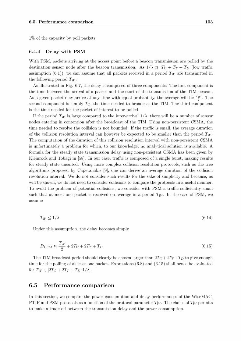
6.5. Performance comparison 103
1% of the capacity by poll packets.
6.4.4 Delay with PSM
With PSM, packets arriving at the access point before a beacon transmission are polled by thedestination sensor node after the beacon transmission. As 1/λ À TC + TT + TD (low trafficassumption (6.1)), we can assume that all packets received in a period TW are transmitted inthe following period TW .
As illustrated in Fig. 6.7, the delay is composed of three components: The first component isthe time between the arrival of a packet and the start of the transmission of the TIM beacon.As a given packet may arrive at any time with equal probability, the average will be TW
2 . Thesecond component is simply TC , the time needed to broadcast the TIM. The third componentis the time needed for the packet of interest to be polled.
If the period TW is large compared to the inter-arrival 1/λ, there will be a number of sensornodes entering in contention after the broadcast of the TIM. Using non-persistent CSMA, thetime needed to resolve the collision is not bounded. If the traffic is small, the average durationof the collision resolution interval can however be expected to be smaller than the period TW .The computation of the duration of this collision resolution interval with non-persistent CSMAis unfortunately a problem for which, to our knowledge, no analytical solution is available. Aformula for the steady state transmission delay using non-persistent CSMA has been given byKleinrock and Tobagi in [58]. In our case, traffic is composed of a single burst, making resultsfor steady state unsuited. Using more complex collision resolution protocols, such as the treealgorithms proposed by Capetanakis [9], one can derive an average duration of the collisionresolution interval. We do not consider such results for the sake of simplicity and because, aswill be shown, we do not need to consider collisions to compare the protocols in a useful manner.To avoid the problem of potential collisions, we consider with PSM a traffic sufficiently smallsuch that at most one packet is received on average in a period TW . In the case of PSM, weassume
TW ≤ 1/λ (6.14)
Under this assumption, the delay becomes simply
DPSM ≈ TW
2+ 2TC + 2TT + TD (6.15)
The TIM broadcast period should clearly be chosen larger than 2TC +2TT +TD to give enoughtime for the polling of at least one packet. Expressions (6.8) and (6.15) shall hence be evaluatedfor TW ∈ [2TC + 2TT + TD; 1/λ].
6.5 Performance comparison
In this section, we compare the power consumption and delay performances of the WiseMAC,PTIP and PSM protocols as a function of the protocol parameter TW . The choice of TW permitsto make a trade-off between the transmission delay and the power consumption.
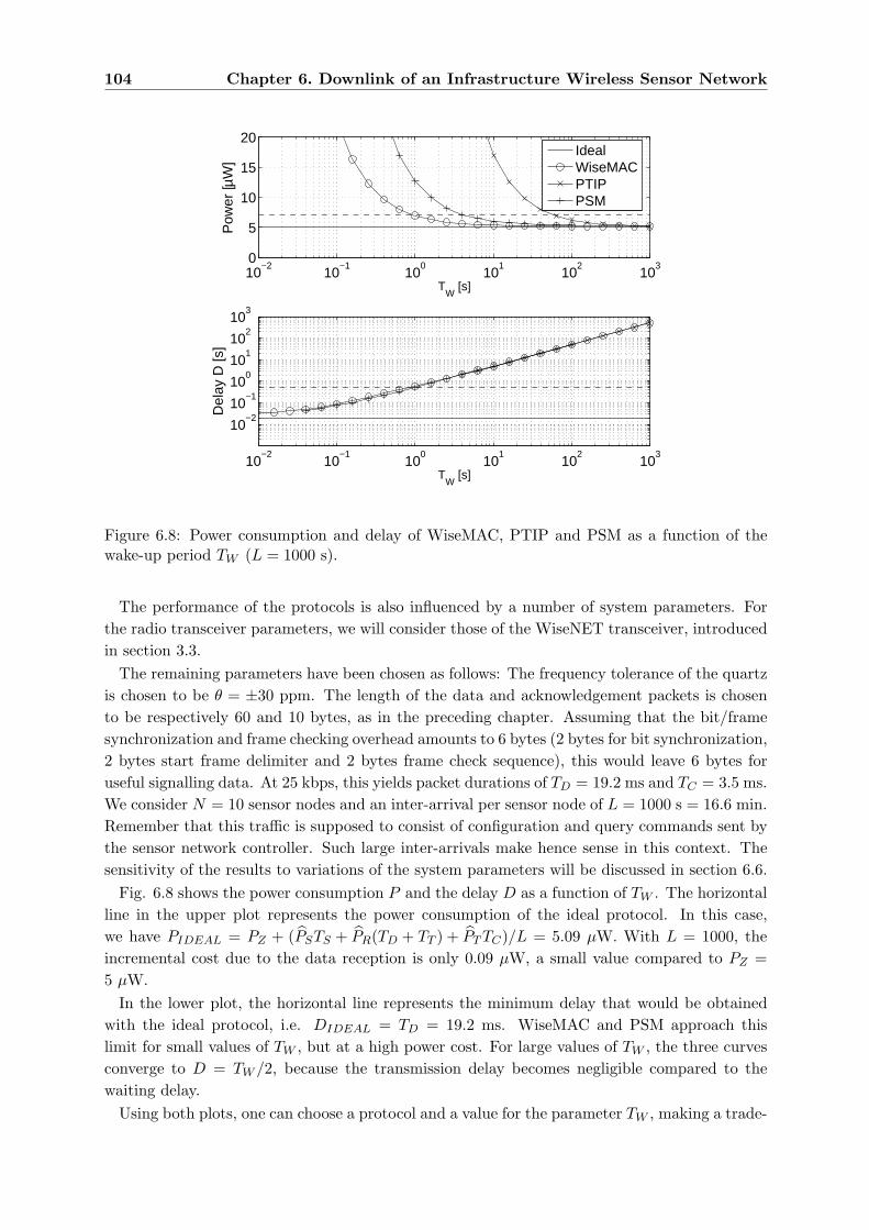
104 Chapter 6. Downlink of an Infrastructure Wireless Sensor Network
10−2
10−1
100
101
102
103
0
5
10
15
20
TW
[s]
Pow
er [µ
W]
IdealWiseMACPTIPPSM
10−2
10−1
100
101
102
103
10−2
10−1
100
101
102
103
TW
[s]
Del
ay D
[s]
Figure 6.8: Power consumption and delay of WiseMAC, PTIP and PSM as a function of thewake-up period TW (L = 1000 s).
The performance of the protocols is also influenced by a number of system parameters. Forthe radio transceiver parameters, we will consider those of the WiseNET transceiver, introducedin section 3.3.
The remaining parameters have been chosen as follows: The frequency tolerance of the quartzis chosen to be θ = ±30 ppm. The length of the data and acknowledgement packets is chosento be respectively 60 and 10 bytes, as in the preceding chapter. Assuming that the bit/framesynchronization and frame checking overhead amounts to 6 bytes (2 bytes for bit synchronization,2 bytes start frame delimiter and 2 bytes frame check sequence), this would leave 6 bytes foruseful signalling data. At 25 kbps, this yields packet durations of TD = 19.2 ms and TC = 3.5 ms.We consider N = 10 sensor nodes and an inter-arrival per sensor node of L = 1000 s = 16.6 min.Remember that this traffic is supposed to consist of configuration and query commands sent bythe sensor network controller. Such large inter-arrivals make hence sense in this context. Thesensitivity of the results to variations of the system parameters will be discussed in section 6.6.
Fig. 6.8 shows the power consumption P and the delay D as a function of TW . The horizontalline in the upper plot represents the power consumption of the ideal protocol. In this case,we have PIDEAL = PZ + (PSTS + PR(TD + TT ) + PT TC)/L = 5.09 µW. With L = 1000, theincremental cost due to the data reception is only 0.09 µW, a small value compared to PZ =5 µW.
In the lower plot, the horizontal line represents the minimum delay that would be obtainedwith the ideal protocol, i.e. DIDEAL = TD = 19.2 ms. WiseMAC and PSM approach thislimit for small values of TW , but at a high power cost. For large values of TW , the three curvesconverge to D = TW /2, because the transmission delay becomes negligible compared to thewaiting delay.
Using both plots, one can choose a protocol and a value for the parameter TW , making a trade-
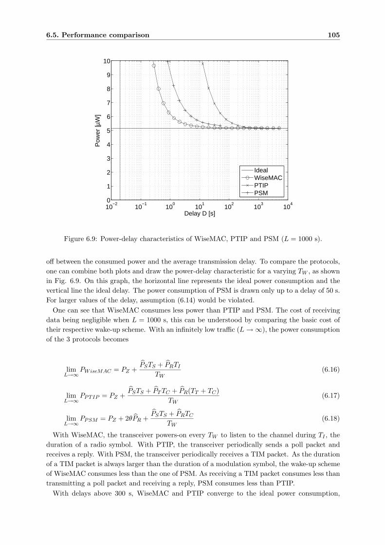
6.5. Performance comparison 105
10−2
10−1
100
101
102
103
104
0
1
2
3
4
5
6
7
8
9
10
Delay D [s]
Pow
er [µ
W]
IdealWiseMACPTIPPSM
Figure 6.9: Power-delay characteristics of WiseMAC, PTIP and PSM (L = 1000 s).
off between the consumed power and the average transmission delay. To compare the protocols,one can combine both plots and draw the power-delay characteristic for a varying TW , as shownin Fig. 6.9. On this graph, the horizontal line represents the ideal power consumption and thevertical line the ideal delay. The power consumption of PSM is drawn only up to a delay of 50 s.For larger values of the delay, assumption (6.14) would be violated.
One can see that WiseMAC consumes less power than PTIP and PSM. The cost of receivingdata being negligible when L = 1000 s, this can be understood by comparing the basic cost oftheir respective wake-up scheme. With an infinitely low traffic (L →∞), the power consumptionof the 3 protocols becomes
limL→∞
PWiseMAC = PZ +PSTS + PRTI
TW(6.16)
limL→∞
PPTIP = PZ +PSTS + PT TC + PR(TT + TC)
TW(6.17)
limL→∞
PPSM = PZ + 2θPR +PSTS + PRTC
TW(6.18)
With WiseMAC, the transceiver powers-on every TW to listen to the channel during TI , theduration of a radio symbol. With PTIP, the transceiver periodically sends a poll packet andreceives a reply. With PSM, the transceiver periodically receives a TIM packet. As the durationof a TIM packet is always larger than the duration of a modulation symbol, the wake-up schemeof WiseMAC consumes less than the one of PSM. As receiving a TIM packet consumes less thantransmitting a poll packet and receiving a reply, PSM consumes less than PTIP.
With delays above 300 s, WiseMAC and PTIP converge to the ideal power consumption,
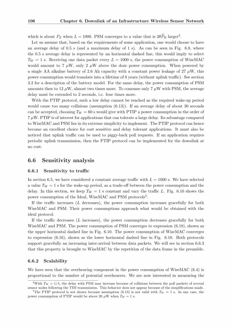
106 Chapter 6. Downlink of an Infrastructure Wireless Sensor Network
which is about PZ when L = 1000. PSM converges to a value that is 2θPR larger2.Let us assume that, based on the requirements of some application, one would choose to have
an average delay of 0.5 s (and a maximum delay of 1 s). As can be seen in Fig. 6.8, wherethe 0.5 s average delay is represented by an horizontal dashed line, this would imply to selectTW = 1 s. Receiving one data packet every L = 1000 s, the power consumption of WiseMACwould amount to 7 µW, only 2 µW above the doze power consumption. When powered bya single AA alkaline battery of 2.6 Ah capacity with a constant power leakage of 27 µW, thispower consumption would translate into a lifetime of 8 years (without uplink traffic). See section3.2 for a description of the battery model. For the same delay, the power consumption of PSMamounts then to 12 µW, almost two times more. To consume only 7 µW with PSM, the averagedelay must be extended to 2 seconds, i.e. four times more.
With the PTIP protocol, such a low delay cannot be reached as the required wake-up periodwould cause too many collisions (assumption (6.13)). If an average delay of about 30 secondscan be accepted, choosing TW = 60 s would give with PTIP a power consumption in the order of7 µW. PTIP is of interest for applications that can tolerate a large delay. Its advantage comparedto WiseMAC and PSM lies in its extreme simplicity to implement. The PTIP protocol can hencebecome an excellent choice for cost sensitive and delay tolerant applications. It must also benoticed that uplink traffic can be used to piggy-back poll requests. If an application requiresperiodic uplink transmission, then the PTIP protocol can be implemented for the downlink atno cost.
6.6 Sensitivity analysis
6.6.1 Sensitivity to traffic
In section 6.5, we have considered a constant average traffic with L = 1000 s. We have selecteda value TW = 1 s for the wake-up period, as a trade-off between the power consumption and thedelay. In this section, we keep TW = 1 s constant and vary the traffic L. Fig. 6.10 shows thepower consumption of the Ideal, WiseMAC and PSM protocols3.
If the traffic increases (L decreases), the power consumption increases gracefully for bothWiseMAC and PSM. Their power consumptions approach what would be obtained with theideal protocol.
If the traffic decreases (L increases), the power consumption decreases gracefully for bothWiseMAC and PSM. The power consumption of PSM converges to expression (6.18), shown asthe upper horizontal dashed line in Fig. 6.10. The power consumption of WiseMAC convergesto expression (6.16), shown as the lower horizontal dashed line in Fig. 6.10. Both protocolssupport gracefully an increasing inter-arrival between data packets. We will see in section 6.6.3that this property is brought to WiseMAC by the repetition of the data frame in the preamble.
6.6.2 Scalability
We have seen that the overhearing component in the power consumption of WiseMAC (6.4) isproportional to the number of potential overhearers. We are now interested in measuring the
2With TW > 1/λ, the delay with PSM may increase because of collisions between the poll packets of severalsensor nodes following the TIM transmission. This behavior does not appear because of the simplifications made.
3The PTIP protocol is not shown because assumption (6.13) is not valid with TW = 1 s. In any case, thepower consumption of PTIP would be above 20 µW when TW = 1 s.
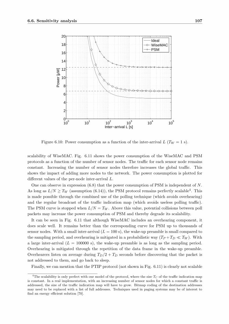
6.6. Sensitivity analysis 107
100
101
102
103
104
105
0
2
4
6
8
10
12
14
16
18
20
Inter−arrival L [s]
Pow
er [µ
W]
IdealWiseMACPSM
Figure 6.10: Power consumption as a function of the inter-arrival L (TW = 1 s).
scalability of WiseMAC. Fig. 6.11 shows the power consumption of the WiseMAC and PSMprotocols as a function of the number of sensor nodes. The traffic for each sensor node remainsconstant. Increasing the number of sensor nodes therefore increases the global traffic. Thisshows the impact of adding more nodes to the network. The power consumption is plotted fordifferent values of the per-node inter-arrival L.
One can observe in expression (6.8) that the power consumption of PSM is independent of N .As long as L/N ≥ TW (assumption (6.14)), the PSM protocol remains perfectly scalable4. Thisis made possible through the combined use of the polling technique (which avoids overhearing)and the regular broadcast of the traffic indication map (which avoids useless polling traffic).The PSM curve is stopped when L/N = TW . Above this value, potential collisions between pollpackets may increase the power consumption of PSM and thereby degrade its scalability.
It can be seen in Fig. 6.11 that although WiseMAC includes an overhearing component, itdoes scale well. It remains better than the corresponding curve for PSM up to thousands ofsensor nodes. With a small inter-arrival (L = 100 s), the wake-up preamble is small compared tothe sampling period, and overhearing is mitigated in a probabilistic way (TP +TD ¿ TW ). Witha large inter-arrival (L = 100000 s), the wake-up preamble is as long as the sampling period.Overhearing is mitigated through the repetition of the data frame in the wake-up preamble.Overhearers listen on average during TD/2 + TD seconds before discovering that the packet isnot addressed to them, and go back to sleep.
Finally, we can mention that the PTIP protocol (not shown in Fig. 6.11) is clearly not scalable
4The scalability is only perfect with our model of the protocol, where the size TC of the traffic indication mapis constant. In a real implementation, with an increasing number of sensor nodes for which a constant traffic isaddressed, the size of the traffic indication map will have to grow. Bitmap coding of the destination addressesmay need to be replaced with a list of full addresses. Techniques used in paging systems may be of interest tofind an energy efficient solution [70].
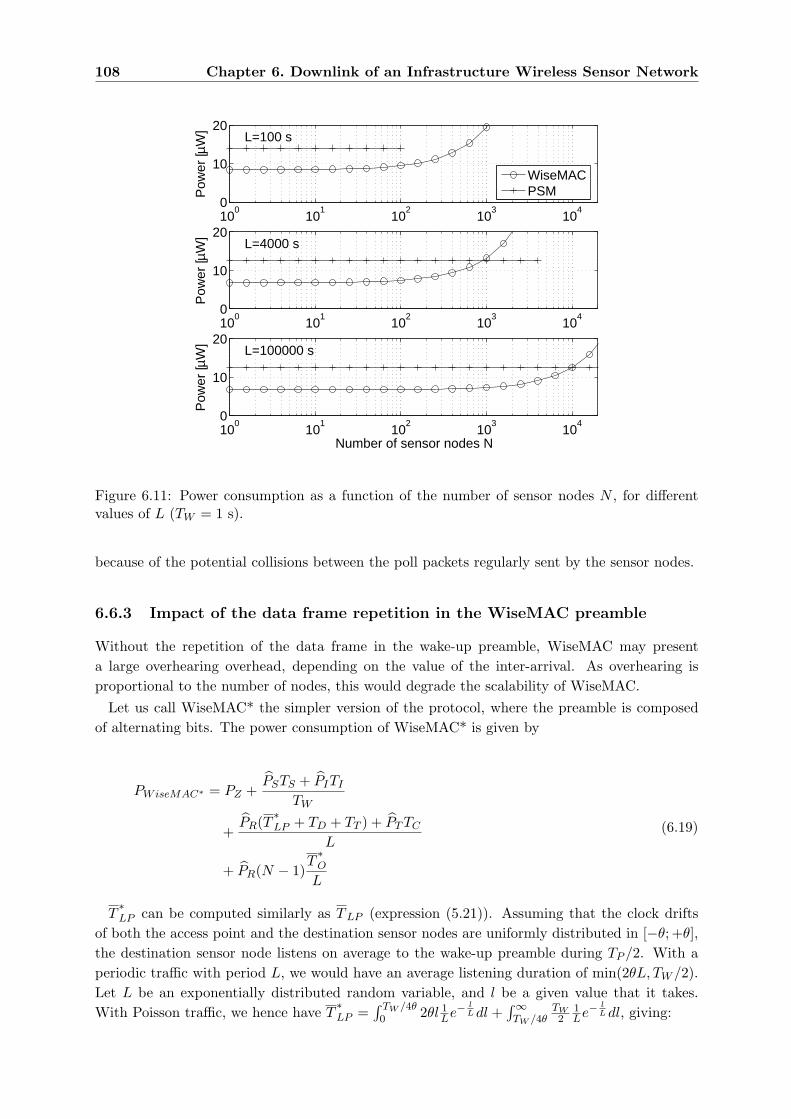
108 Chapter 6. Downlink of an Infrastructure Wireless Sensor Network
100
101
102
103
104
0
10
20L=100 s
Pow
er [µ
W]
WiseMACPSM
100
101
102
103
104
0
10
20L=4000 s
Pow
er [µ
W]
100
101
102
103
104
0
10
20
Number of sensor nodes N
L=100000 s
Pow
er [µ
W]
Figure 6.11: Power consumption as a function of the number of sensor nodes N , for differentvalues of L (TW = 1 s).
because of the potential collisions between the poll packets regularly sent by the sensor nodes.
6.6.3 Impact of the data frame repetition in the WiseMAC preamble
Without the repetition of the data frame in the wake-up preamble, WiseMAC may presenta large overhearing overhead, depending on the value of the inter-arrival. As overhearing isproportional to the number of nodes, this would degrade the scalability of WiseMAC.
Let us call WiseMAC* the simpler version of the protocol, where the preamble is composedof alternating bits. The power consumption of WiseMAC* is given by
PWiseMAC∗ = PZ +PSTS + PITI
TW
+PR(T ∗LP + TD + TT ) + PT TC
L
+ PR(N − 1)T∗O
L
(6.19)
T∗LP can be computed similarly as TLP (expression (5.21)). Assuming that the clock drifts
of both the access point and the destination sensor nodes are uniformly distributed in [−θ; +θ],the destination sensor node listens on average to the wake-up preamble during TP /2. With aperiodic traffic with period L, we would have an average listening duration of min(2θL, TW /2).Let L be an exponentially distributed random variable, and l be a given value that it takes.With Poisson traffic, we hence have T
∗LP =
∫ TW /4θ0 2θl 1
Le−lL dl +
∫∞TW /4θ
TW2
1Le−
lL dl, giving:
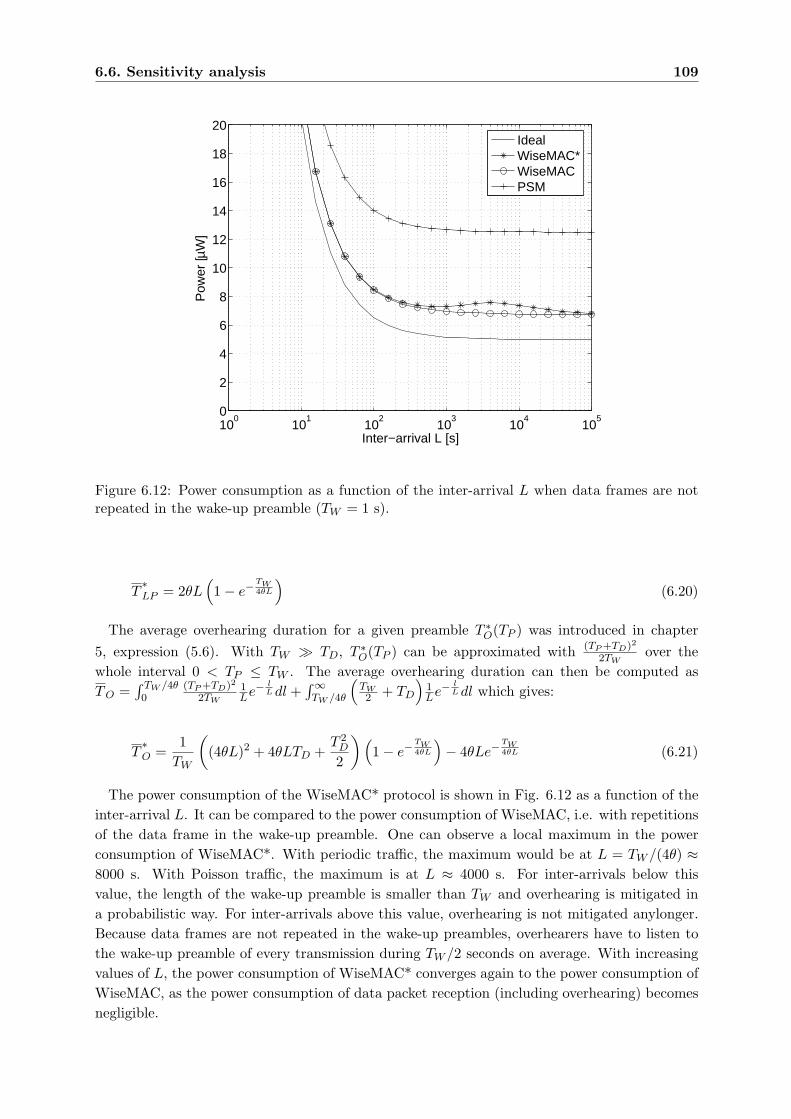
6.6. Sensitivity analysis 109
100
101
102
103
104
105
0
2
4
6
8
10
12
14
16
18
20
Inter−arrival L [s]
Pow
er [µ
W]
IdealWiseMAC*WiseMACPSM
Figure 6.12: Power consumption as a function of the inter-arrival L when data frames are notrepeated in the wake-up preamble (TW = 1 s).
T∗LP = 2θL
(1− e−
TW4θL
)(6.20)
The average overhearing duration for a given preamble T ∗O(TP ) was introduced in chapter5, expression (5.6). With TW À TD, T ∗O(TP ) can be approximated with (TP +TD)2
2TWover the
whole interval 0 < TP ≤ TW . The average overhearing duration can then be computed asTO =
∫ TW /4θ0
(TP +TD)2
2TW
1Le−
lL dl +
∫∞TW /4θ
(TW2 + TD
)1Le−
lL dl which gives:
T∗O =
1TW
((4θL)2 + 4θLTD +
T 2D
2
)(1− e−
TW4θL
)− 4θLe−
TW4θL (6.21)
The power consumption of the WiseMAC* protocol is shown in Fig. 6.12 as a function of theinter-arrival L. It can be compared to the power consumption of WiseMAC, i.e. with repetitionsof the data frame in the wake-up preamble. One can observe a local maximum in the powerconsumption of WiseMAC*. With periodic traffic, the maximum would be at L = TW /(4θ) ≈8000 s. With Poisson traffic, the maximum is at L ≈ 4000 s. For inter-arrivals below thisvalue, the length of the wake-up preamble is smaller than TW and overhearing is mitigated ina probabilistic way. For inter-arrivals above this value, overhearing is not mitigated anylonger.Because data frames are not repeated in the wake-up preambles, overhearers have to listen tothe wake-up preamble of every transmission during TW /2 seconds on average. With increasingvalues of L, the power consumption of WiseMAC* converges again to the power consumption ofWiseMAC, as the power consumption of data packet reception (including overhearing) becomesnegligible.
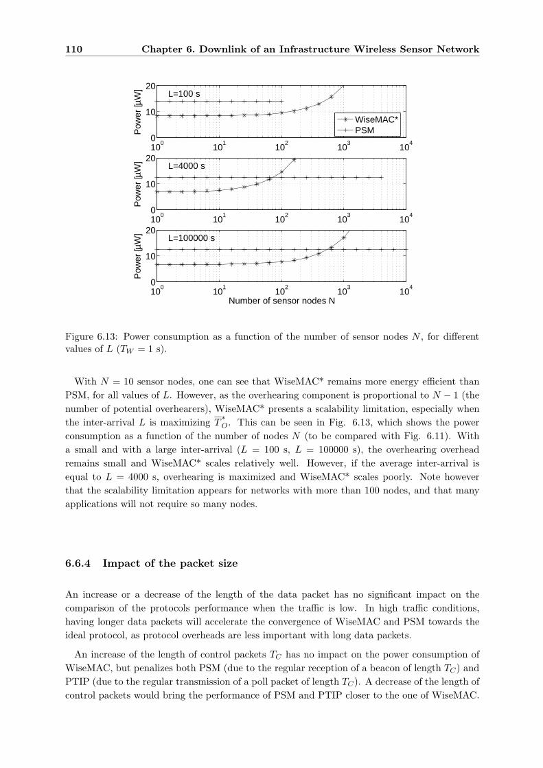
110 Chapter 6. Downlink of an Infrastructure Wireless Sensor Network
100
101
102
103
104
0
10
20L=100 s
Pow
er [µ
W]
WiseMAC*PSM
100
101
102
103
104
0
10
20L=4000 s
Pow
er [µ
W]
100
101
102
103
104
0
10
20
Number of sensor nodes N
L=100000 s
Pow
er [µ
W]
Figure 6.13: Power consumption as a function of the number of sensor nodes N , for differentvalues of L (TW = 1 s).
With N = 10 sensor nodes, one can see that WiseMAC* remains more energy efficient thanPSM, for all values of L. However, as the overhearing component is proportional to N − 1 (thenumber of potential overhearers), WiseMAC* presents a scalability limitation, especially whenthe inter-arrival L is maximizing T
∗O. This can be seen in Fig. 6.13, which shows the power
consumption as a function of the number of nodes N (to be compared with Fig. 6.11). Witha small and with a large inter-arrival (L = 100 s, L = 100000 s), the overhearing overheadremains small and WiseMAC* scales relatively well. However, if the average inter-arrival isequal to L = 4000 s, overhearing is maximized and WiseMAC* scales poorly. Note howeverthat the scalability limitation appears for networks with more than 100 nodes, and that manyapplications will not require so many nodes.
6.6.4 Impact of the packet size
An increase or a decrease of the length of the data packet has no significant impact on thecomparison of the protocols performance when the traffic is low. In high traffic conditions,having longer data packets will accelerate the convergence of WiseMAC and PSM towards theideal protocol, as protocol overheads are less important with long data packets.
An increase of the length of control packets TC has no impact on the power consumption ofWiseMAC, but penalizes both PSM (due to the regular reception of a beacon of length TC) andPTIP (due to the regular transmission of a poll packet of length TC). A decrease of the length ofcontrol packets would bring the performance of PSM and PTIP closer to the one of WiseMAC.
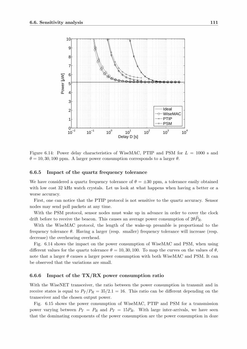
6.6. Sensitivity analysis 111
10−2
10−1
100
101
102
103
104
0
1
2
3
4
5
6
7
8
9
10
Delay D [s]
Pow
er [µ
W]
IdealWiseMACPTIPPSM
Figure 6.14: Power delay characteristics of WiseMAC, PTIP and PSM for L = 1000 s andθ = 10, 30, 100 ppm. A larger power consumption corresponds to a larger θ.
6.6.5 Impact of the quartz frequency tolerance
We have considered a quartz frequency tolerance of θ = ±30 ppm, a tolerance easily obtainedwith low cost 32 kHz watch crystals. Let us look at what happens when having a better or aworse accuracy.
First, one can notice that the PTIP protocol is not sensitive to the quartz accuracy. Sensornodes may send poll packets at any time.
With the PSM protocol, sensor nodes must wake up in advance in order to cover the clockdrift before to receive the beacon. This causes an average power consumption of 2θPR.
With the WiseMAC protocol, the length of the wake-up preamble is proportional to thefrequency tolerance θ. Having a larger (resp. smaller) frequency tolerance will increase (resp.decrease) the overhearing overhead.
Fig. 6.14 shows the impact on the power consumption of WiseMAC and PSM, when usingdifferent values for the quartz tolerance θ = 10, 30, 100. To map the curves on the values of θ,note that a larger θ causes a larger power consumption with both WiseMAC and PSM. It canbe observed that the variations are small.
6.6.6 Impact of the TX/RX power consumption ratio
With the WiseNET transceiver, the ratio between the power consumption in transmit and inreceive states is equal to PT /PR = 35/2.1 = 16. This ratio can be different depending on thetransceiver and the chosen output power.
Fig. 6.15 shows the power consumption of WiseMAC, PTIP and PSM for a transmissionpower varying between PT = PR and PT = 15PR. With large inter-arrivals, we have seenthat the dominating components of the power consumption are the power consumption in doze
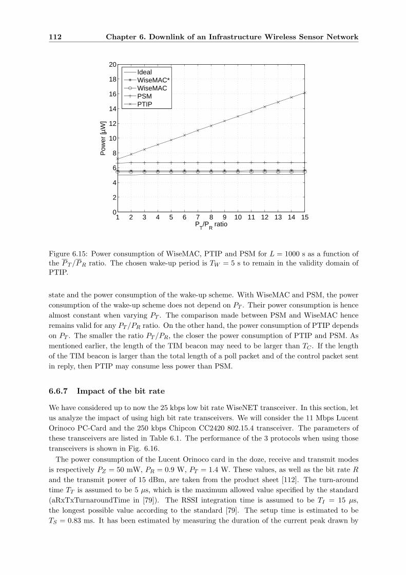
112 Chapter 6. Downlink of an Infrastructure Wireless Sensor Network
1 2 3 4 5 6 7 8 9 10 11 12 13 14 150
2
4
6
8
10
12
14
16
18
20
Pow
er [µ
W]
PT/P
R ratio
IdealWiseMAC*WiseMACPSMPTIP
Figure 6.15: Power consumption of WiseMAC, PTIP and PSM for L = 1000 s as a function ofthe P T /PR ratio. The chosen wake-up period is TW = 5 s to remain in the validity domain ofPTIP.
state and the power consumption of the wake-up scheme. With WiseMAC and PSM, the powerconsumption of the wake-up scheme does not depend on PT . Their power consumption is hencealmost constant when varying PT . The comparison made between PSM and WiseMAC henceremains valid for any PT /PR ratio. On the other hand, the power consumption of PTIP dependson PT . The smaller the ratio PT /PR, the closer the power consumption of PTIP and PSM. Asmentioned earlier, the length of the TIM beacon may need to be larger than TC . If the lengthof the TIM beacon is larger than the total length of a poll packet and of the control packet sentin reply, then PTIP may consume less power than PSM.
6.6.7 Impact of the bit rate
We have considered up to now the 25 kbps low bit rate WiseNET transceiver. In this section, letus analyze the impact of using high bit rate transceivers. We will consider the 11 Mbps LucentOrinoco PC-Card and the 250 kbps Chipcon CC2420 802.15.4 transceiver. The parameters ofthese transceivers are listed in Table 6.1. The performance of the 3 protocols when using thosetransceivers is shown in Fig. 6.16.
The power consumption of the Lucent Orinoco card in the doze, receive and transmit modesis respectively PZ = 50 mW, PR = 0.9 W, PT = 1.4 W. These values, as well as the bit rate R
and the transmit power of 15 dBm, are taken from the product sheet [112]. The turn-aroundtime TT is assumed to be 5 µs, which is the maximum allowed value specified by the standard(aRxTxTurnaroundTime in [79]). The RSSI integration time is assumed to be TI = 15 µs,the longest possible value according to the standard [79]. The setup time is estimated to beTS = 0.83 ms. It has been estimated by measuring the duration of the current peak drawn by
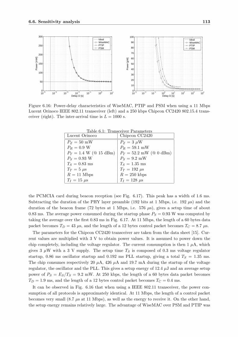
6.6. Sensitivity analysis 113
10−5
10−4
10−3
10−2
10−1
100
101
0
50
100
150
200
250
300
Delay D [s]
Pow
er [m
W]
IdealWiseMACPTIPPSM
10−3
10−2
10−1
100
101
102
103
104
0
10
20
30
40
50
60
70
80
90
100
Delay D [s]
Pow
er [µ
W]
IdealWiseMACPTIPPSM
Figure 6.16: Power-delay characteristics of WiseMAC, PTIP and PSM when using a 11 MbpsLucent Orinoco IEEE 802.11 transceiver (left) and a 250 kbps Chipcon CC2420 802.15.4 trans-ceiver (right). The inter-arrival time is L = 1000 s.
Table 6.1: Transceiver ParametersLucent Orinoco Chipcon CC2420PZ = 50 mW PZ = 3 µWPR = 0.9 W PR = 59.1 mWPT = 1.4 W (@ 15 dBm) PT = 52.2 mW (@ 0 dBm)PS = 0.93 W PS = 9.2 mWTS = 0.83 ms TS = 1.35 msTT = 5 µs TT = 192 µsR = 11 Mbps R = 250 kbpsTI = 15 µs TI = 128 µs
the PCMCIA card during beacon reception (see Fig. 6.17). This peak has a width of 1.6 ms.Subtracting the duration of the PHY layer preamble (192 bits at 1 Mbps, i.e. 192 µs) and theduration of the beacon frame (72 bytes at 1 Mbps, i.e. 576 µs), gives a setup time of about0.83 ms. The average power consumed during the startup phase PS = 0.93 W was computed bytaking the average over the first 0.83 ms in Fig. 6.17. At 11 Mbps, the length of a 60 bytes datapacket becomes TD = 43 µs, and the length of a 12 bytes control packet becomes TC = 8.7 µs.
The parameters for the Chipcon CC2420 transceiver are taken from the data sheet [15]. Cur-rent values are multiplied with 3 V to obtain power values. It is assumed to power down thechip completely, including the voltage regulator. The current consumption is then 1 µA, whichgives 3 µW with a 3 V supply. The setup time TS is composed of 0.3 ms voltage regulatorstartup, 0.86 ms oscillator startup and 0.192 ms PLL startup, giving a total TS = 1.35 ms.The chip consumes respectively 20 µA, 426 µA and 19.7 mA during the startup of the voltageregulator, the oscillator and the PLL. This gives a setup energy of 12.4 µJ and an average setuppower of PS = ES/TS = 9.2 mW. At 250 kbps, the length of a 60 bytes data packet becomesTD = 1.9 ms, and the length of a 12 bytes control packet becomes TC = 0.4 ms.
It can be observed in Fig. 6.16 that when using a IEEE 802.11 transceiver, the power con-sumption of all protocols is approximately identical. At 11 Mbps, the length of a control packetbecomes very small (8.7 µs at 11 Mbps), as well as the energy to receive it. On the other hand,the setup energy remains relatively large. The advantage of WiseMAC over PSM and PTIP was
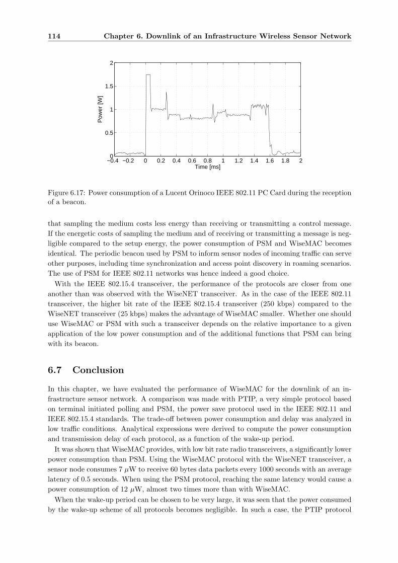
114 Chapter 6. Downlink of an Infrastructure Wireless Sensor Network
−0.4 −0.2 0 0.2 0.4 0.6 0.8 1 1.2 1.4 1.6 1.8 20
0.5
1
1.5
2
Time [ms]
Pow
er [W
]
Figure 6.17: Power consumption of a Lucent Orinoco IEEE 802.11 PC Card during the receptionof a beacon.
that sampling the medium costs less energy than receiving or transmitting a control message.If the energetic costs of sampling the medium and of receiving or transmitting a message is neg-ligible compared to the setup energy, the power consumption of PSM and WiseMAC becomesidentical. The periodic beacon used by PSM to inform sensor nodes of incoming traffic can serveother purposes, including time synchronization and access point discovery in roaming scenarios.The use of PSM for IEEE 802.11 networks was hence indeed a good choice.
With the IEEE 802.15.4 transceiver, the performance of the protocols are closer from oneanother than was observed with the WiseNET transceiver. As in the case of the IEEE 802.11transceiver, the higher bit rate of the IEEE 802.15.4 transceiver (250 kbps) compared to theWiseNET transceiver (25 kbps) makes the advantage of WiseMAC smaller. Whether one shoulduse WiseMAC or PSM with such a transceiver depends on the relative importance to a givenapplication of the low power consumption and of the additional functions that PSM can bringwith its beacon.
6.7 Conclusion
In this chapter, we have evaluated the performance of WiseMAC for the downlink of an in-frastructure sensor network. A comparison was made with PTIP, a very simple protocol basedon terminal initiated polling and PSM, the power save protocol used in the IEEE 802.11 andIEEE 802.15.4 standards. The trade-off between power consumption and delay was analyzed inlow traffic conditions. Analytical expressions were derived to compute the power consumptionand transmission delay of each protocol, as a function of the wake-up period.
It was shown that WiseMAC provides, with low bit rate radio transceivers, a significantly lowerpower consumption than PSM. Using the WiseMAC protocol with the WiseNET transceiver, asensor node consumes 7 µW to receive 60 bytes data packets every 1000 seconds with an averagelatency of 0.5 seconds. When using the PSM protocol, reaching the same latency would cause apower consumption of 12 µW, almost two times more than with WiseMAC.
When the wake-up period can be chosen to be very large, it was seen that the power consumedby the wake-up scheme of all protocols becomes negligible. In such a case, the PTIP protocol
6.7. Conclusion 115
becomes attractive as well, because of its implementation simplicity.With high bit rate transceivers, it was seen that the power consumption of all protocols con-
verge to the power consumption of the periodic wake-up. With an increasing bit rate, the addi-tional activity specific to each protocol becomes negligible. Choosing PSM instead of WiseMACbecomes attractive because of the additional functions that a beacon can offer.

Chapter 7
Experimentation
7.1 Introduction
This chapter presents experimental results obtained with an implementation of the WiseMACprotocol. After a presentation of the used hardware platform, the operation of the WiseMACprotocol will be illustrated with oscilloscope traces. Average power consumption and delaymeasurements are finally presented.
7.2 Hardware platform
In order to advance in parallel with the finalization of the WiseNET SoC, the implementationof the WiseMAC communication protocol investigated in this dissertation was first made on atwo-chips platform composed of the XE88LC06A [124] microcontroller and the XE1203F [127]FSK radio transceiver. Both chips are products from Xemics, a spin-off company of CSEM.
7.2.1 Microcontroller
The XE88LC06A [124] is an 8-bit microcontroller designed for wireless communication applica-tions. It is based on the same CoolRISC 816 core [123] used in the WiseNET SoC, facilitatingcode porting towards the WiseNET SoC platform.
The architecture of the XE88LC06A microcontroller is illustrated in Fig. 7.1. The computerarchitecture of the CoolRISC 816 core is of the Harvard type [123], with a physically separatedstorage for instructions and data. The size of the instruction memory is of 8192 instructions.As instructions have a width of 22 bits, this corresponds to 22 kbytes. The size of the datamemory is only 512 bytes. When programming in C with the gcc CoolRISC compiler, one mustreserve a zone on the top of the data memory for the software stack, reducing further the spaceavailable for program variables.
When compared to the classical Von Neumann architecture [119], where data and instructionsare stored in the same memory, the Harvard architecture presents the advantage of allowingthe execution of one instruction per clock cycle. As power consumption is proportional toclock frequency, the Harvard architecture permits a lower power consumption per MIPS. Thedisadvantage of the Harvard architecture is to prevent the reading of constants directly from theprogram memory. Many algorithms (e.g. ciphers and CRCs implementations) are based on theuse of lookup tables with 256 entries to map a byte onto the result of some complex operation.
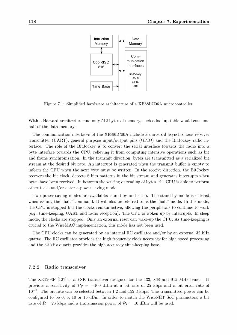
118 Chapter 7. Experimentation
CoolRISC816
IntructionMemory
Time Base
DataMemory
Com -municationInterfaces
BitJockeyUARTGPIO
etc
Figure 7.1: Simplified hardware architecture of a XE88LC06A microcontroller.
With a Harvard architecture and only 512 bytes of memory, such a lookup table would consumehalf of the data memory.
The communication interfaces of the XE88LC06A include a universal asynchronous receivertransmitter (UART), general purpose input/output pins (GPIO) and the BitJockey radio in-terface. The role of the BitJockey is to convert the serial interface towards the radio into abyte interface towards the CPU, relieving it from computing intensive operations such as bitand frame synchronization. In the transmit direction, bytes are transmitted as a serialized bitstream at the desired bit rate. An interrupt is generated when the transmit buffer is empty toinform the CPU when the next byte must be written. In the receive direction, the BitJockeyrecovers the bit clock, detects 8 bits patterns in the bit stream and generates interrupts whenbytes have been received. In between the writing or reading of bytes, the CPU is able to performother tasks and/or enter a power saving mode.
Two power-saving modes are available: stand-by and sleep. The stand-by mode is enteredwhen issuing the ”halt” command. It will also be referred to as the ”halt” mode. In this mode,the CPU is stopped but the clocks remain active, allowing the peripherals to continue to work(e.g. time-keeping, UART and radio reception). The CPU is woken up by interrupts. In sleepmode, the clocks are stopped. Only an external reset can wake-up the CPU. As time-keeping iscrucial to the WiseMAC implementation, this mode has not been used.
The CPU clocks can be generated by an internal RC oscillator and/or by an external 32 kHzquartz. The RC oscillator provides the high frequency clock necessary for high speed processingand the 32 kHz quartz provides the high accuracy time-keeping base.
7.2.2 Radio transceiver
The XE1203F [127] is a FSK transceiver designed for the 433, 868 and 915 MHz bands. Itprovides a sensitivity of PS = −109 dBm at a bit rate of 25 kbps and a bit error rate of10−3. The bit rate can be selected between 1.2 and 152.3 kbps. The transmitted power can beconfigured to be 0, 5, 10 or 15 dBm. In order to match the WiseNET SoC parameters, a bitrate of R = 25 kbps and a transmission power of PT = 10 dBm will be used.
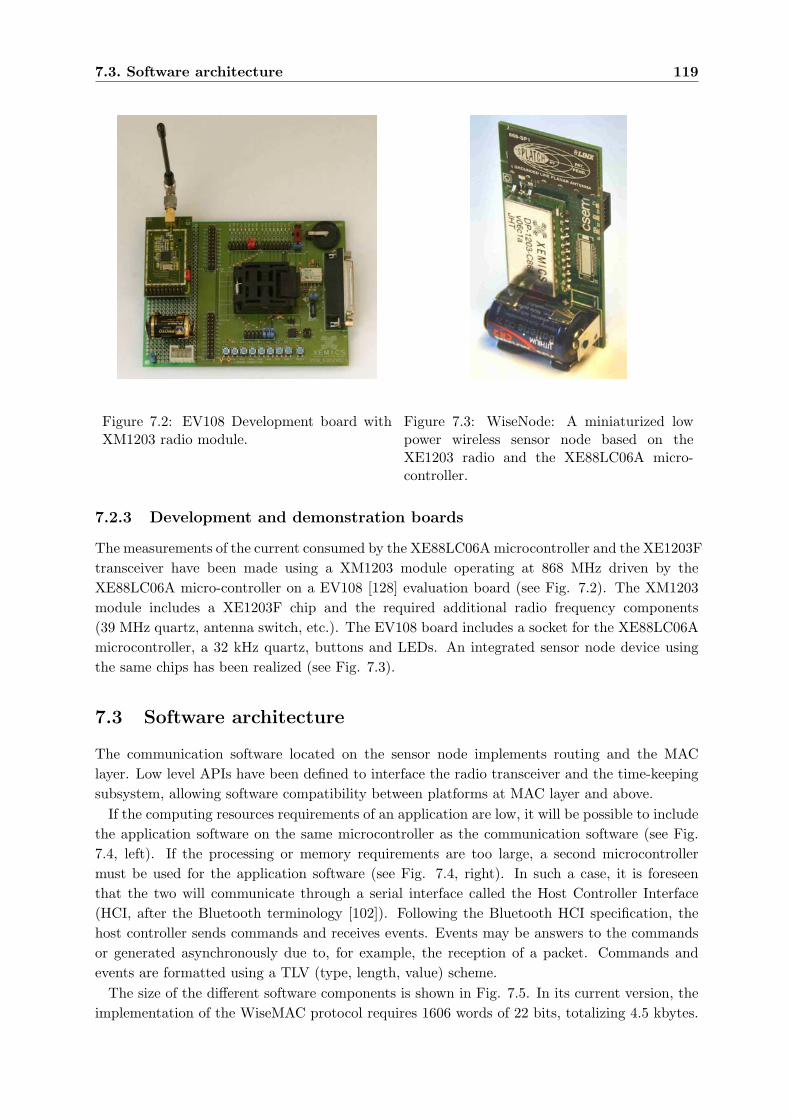
7.3. Software architecture 119
Figure 7.2: EV108 Development board withXM1203 radio module.
Figure 7.3: WiseNode: A miniaturized lowpower wireless sensor node based on theXE1203 radio and the XE88LC06A micro-controller.
7.2.3 Development and demonstration boards
The measurements of the current consumed by the XE88LC06A microcontroller and the XE1203Ftransceiver have been made using a XM1203 module operating at 868 MHz driven by theXE88LC06A micro-controller on a EV108 [128] evaluation board (see Fig. 7.2). The XM1203module includes a XE1203F chip and the required additional radio frequency components(39 MHz quartz, antenna switch, etc.). The EV108 board includes a socket for the XE88LC06Amicrocontroller, a 32 kHz quartz, buttons and LEDs. An integrated sensor node device usingthe same chips has been realized (see Fig. 7.3).
7.3 Software architecture
The communication software located on the sensor node implements routing and the MAClayer. Low level APIs have been defined to interface the radio transceiver and the time-keepingsubsystem, allowing software compatibility between platforms at MAC layer and above.
If the computing resources requirements of an application are low, it will be possible to includethe application software on the same microcontroller as the communication software (see Fig.7.4, left). If the processing or memory requirements are too large, a second microcontrollermust be used for the application software (see Fig. 7.4, right). In such a case, it is foreseenthat the two will communicate through a serial interface called the Host Controller Interface(HCI, after the Bluetooth terminology [102]). Following the Bluetooth HCI specification, thehost controller sends commands and receives events. Events may be answers to the commandsor generated asynchronously due to, for example, the reception of a packet. Commands andevents are formatted using a TLV (type, length, value) scheme.
The size of the different software components is shown in Fig. 7.5. In its current version, theimplementation of the WiseMAC protocol requires 1606 words of 22 bits, totalizing 4.5 kbytes.
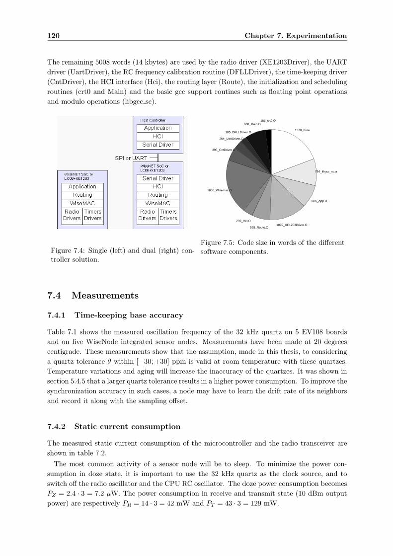
120 Chapter 7. Experimentation
The remaining 5008 words (14 kbytes) are used by the radio driver (XE1203Driver), the UARTdriver (UartDriver), the RC frequency calibration routine (DFLLDriver), the time-keeping driver(CntDriver), the HCI interface (Hci), the routing layer (Route), the initialization and schedulingroutines (crt0 and Main) and the basic gcc support routines such as floating point operationsand modulo operations (libgcc sc).
Figure 7.4: Single (left) and dual (right) con-troller solution.
181_crt0.O 600_Main.O
185_DFLLDriver.O
264_UartDriver.O
395_CntDriver.O
1606_Wisemac.O
292_Hci.O
529_Route.O1092_XE1203Driver.O
686_App.O
784_libgcc_sc.a
1578_Free
Figure 7.5: Code size in words of the differentsoftware components.
7.4 Measurements
7.4.1 Time-keeping base accuracy
Table 7.1 shows the measured oscillation frequency of the 32 kHz quartz on 5 EV108 boardsand on five WiseNode integrated sensor nodes. Measurements have been made at 20 degreescentigrade. These measurements show that the assumption, made in this thesis, to consideringa quartz tolerance θ within [−30;+30] ppm is valid at room temperature with these quartzes.Temperature variations and aging will increase the inaccuracy of the quartzes. It was shown insection 5.4.5 that a larger quartz tolerance results in a higher power consumption. To improve thesynchronization accuracy in such cases, a node may have to learn the drift rate of its neighborsand record it along with the sampling offset.
7.4.2 Static current consumption
The measured static current consumption of the microcontroller and the radio transceiver areshown in table 7.2.
The most common activity of a sensor node will be to sleep. To minimize the power con-sumption in doze state, it is important to use the 32 kHz quartz as the clock source, and toswitch off the radio oscillator and the CPU RC oscillator. The doze power consumption becomesPZ = 2.4 · 3 = 7.2 µW. The power consumption in receive and transmit state (10 dBm outputpower) are respectively PR = 14 · 3 = 42 mW and PT = 43 · 3 = 129 mW.
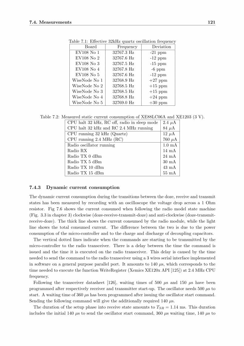
7.4. Measurements 121
Table 7.1: Effective 32kHz quartz oscillation frequencyBoard Frequency Deviation
EV108 No 1 32767.3 Hz -21 ppmEV108 No 2 32767.6 Hz -12 ppmEV108 No 3 32767.5 Hz -15 ppmEV108 No 4 32767.8 Hz -6 ppmEV108 No 5 32767.6 Hz -12 ppm
WiseNode No 1 32768.9 Hz +27 ppmWiseNode No 2 32768.5 Hz +15 ppmWiseNode No 3 32768.5 Hz +15 ppmWiseNode No 4 32768.8 Hz +24 ppmWiseNode No 5 32769.0 Hz +30 ppm
Table 7.2: Measured static current consumption of XE88LC06A and XE1203 (3 V).CPU halt 32 kHz, RC off, radio in sleep mode 2.4 µACPU halt 32 kHz and RC 2.4 MHz running 84 µACPU running 32 kHz (Quartz) 12 µACPU running 2.4 MHz (RC) 760 µARadio oscillator running 1.0 mARadio RX 14 mARadio TX 0 dBm 24 mARadio TX 5 dBm 30 mARadio TX 10 dBm 43 mARadio TX 15 dBm 55 mA
7.4.3 Dynamic current consumption
The dynamic current consumption during the transitions between the doze, receive and transmitstates has been measured by recording with an oscilloscope the voltage drop across a 1 Ohmresistor. Fig 7.6 shows the current consumed when following the radio model state machine(Fig. 3.3 in chapter 3) clockwise (doze-receive-transmit-doze) and anti-clockwise (doze-transmit-receive-doze). The thick line shows the current consumed by the radio module, while the lightline shows the total consumed current. The difference between the two is due to the powerconsumption of the micro-controller and to the charge and discharge of decoupling capacitors.
The vertical dotted lines indicate when the commands are starting to be transmitted by themicro-controller to the radio transceiver. There is a delay between the time the command isissued and the time it is executed on the radio transceiver. This delay is caused by the timeneeded to send the command to the radio transceiver using a 3 wires serial interface implementedin software on a general purpose parallel port. It amounts to 140 µs, which corresponds to thetime needed to execute the function WriteRegister (Xemics XE120x API [125]) at 2.4 MHz CPUfrequency.
Following the transceiver datasheet [126], waiting times of 500 µs and 150 µs have beenprogrammed after respectively receiver and transmitter start-up. The oscillator needs 500 µs tostart. A waiting time of 360 µs has been programmed after issuing the oscillator start command.Sending the following command will give the additionally required 140 µs.
The duration of the setup phase into receive state amounts to TSR = 1.14 ms. This durationincludes the initial 140 µs to send the oscillator start command, 360 µs waiting time, 140 µs to
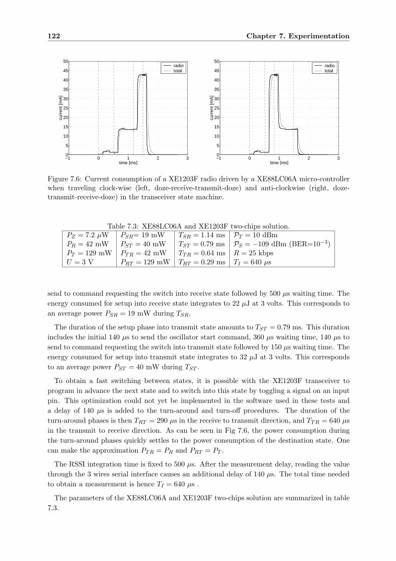
122 Chapter 7. Experimentation
−1 0 1 2 30
5
10
15
20
25
30
35
40
45
50
time [ms]
curr
ent [
mA
]radiototal
−1 0 1 2 30
5
10
15
20
25
30
35
40
45
50
time [ms]
curr
ent [
mA
]
radiototal
Figure 7.6: Current consumption of a XE1203F radio driven by a XE88LC06A micro-controllerwhen traveling clock-wise (left, doze-receive-transmit-doze) and anti-clockwise (right, doze-transmit-receive-doze) in the transceiver state machine.
Table 7.3: XE88LC06A and XE1203F two-chips solution.PZ = 7.2 µW PSR= 19 mW TSR = 1.14 ms PT = 10 dBmPR = 42 mW PST = 40 mW TST = 0.79 ms PS = −109 dBm (BER=10−3)PT = 129 mW PTR = 42 mW TTR = 0.64 ms R = 25 kbpsU = 3 V PRT = 129 mW TRT = 0.29 ms TI = 640 µs
send to command requesting the switch into receive state followed by 500 µs waiting time. Theenergy consumed for setup into receive state integrates to 22 µJ at 3 volts. This corresponds toan average power PSR = 19 mW during TSR.
The duration of the setup phase into transmit state amounts to TST = 0.79 ms. This durationincludes the initial 140 µs to send the oscillator start command, 360 µs waiting time, 140 µs tosend to command requesting the switch into transmit state followed by 150 µs waiting time. Theenergy consumed for setup into transmit state integrates to 32 µJ at 3 volts. This correspondsto an average power PST = 40 mW during TST .
To obtain a fast switching between states, it is possible with the XE1203F transceiver toprogram in advance the next state and to switch into this state by toggling a signal on an inputpin. This optimization could not yet be implemented in the software used in these tests anda delay of 140 µs is added to the turn-around and turn-off procedures. The duration of theturn-around phases is then TRT = 290 µs in the receive to transmit direction, and TTR = 640 µsin the transmit to receive direction. As can be seen in Fig 7.6, the power consumption duringthe turn-around phases quickly settles to the power consumption of the destination state. Onecan make the approximation PTR = PR and PRT = PT .
The RSSI integration time is fixed to 500 µs. After the measurement delay, reading the valuethrough the 3 wires serial interface causes an additional delay of 140 µs. The total time neededto obtain a measurement is hence TI = 640 µs .
The parameters of the XE88LC06A and XE1203F two-chips solution are summarized in table7.3.
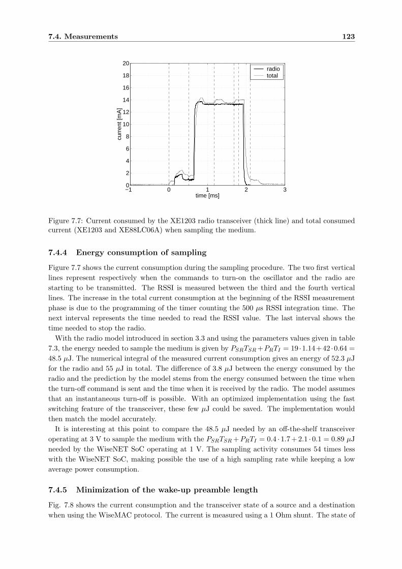
7.4. Measurements 123
−1 0 1 2 30
2
4
6
8
10
12
14
16
18
20
time [ms]
curr
ent [
mA
]
radiototal
Figure 7.7: Current consumed by the XE1203 radio transceiver (thick line) and total consumedcurrent (XE1203 and XE88LC06A) when sampling the medium.
7.4.4 Energy consumption of sampling
Figure 7.7 shows the current consumption during the sampling procedure. The two first verticallines represent respectively when the commands to turn-on the oscillator and the radio arestarting to be transmitted. The RSSI is measured between the third and the fourth verticallines. The increase in the total current consumption at the beginning of the RSSI measurementphase is due to the programming of the timer counting the 500 µs RSSI integration time. Thenext interval represents the time needed to read the RSSI value. The last interval shows thetime needed to stop the radio.
With the radio model introduced in section 3.3 and using the parameters values given in table7.3, the energy needed to sample the medium is given by PSRTSR +PRTI = 19 ·1.14+42 ·0.64 =48.5 µJ. The numerical integral of the measured current consumption gives an energy of 52.3 µJfor the radio and 55 µJ in total. The difference of 3.8 µJ between the energy consumed by theradio and the prediction by the model stems from the energy consumed between the time whenthe turn-off command is sent and the time when it is received by the radio. The model assumesthat an instantaneous turn-off is possible. With an optimized implementation using the fastswitching feature of the transceiver, these few µJ could be saved. The implementation wouldthen match the model accurately.
It is interesting at this point to compare the 48.5 µJ needed by an off-the-shelf transceiveroperating at 3 V to sample the medium with the PSRTSR +PRTI = 0.4 · 1.7+2.1 · 0.1 = 0.89 µJneeded by the WiseNET SoC operating at 1 V. The sampling activity consumes 54 times lesswith the WiseNET SoC, making possible the use of a high sampling rate while keeping a lowaverage power consumption.
7.4.5 Minimization of the wake-up preamble length
Fig. 7.8 shows the current consumption and the transceiver state of a source and a destinationwhen using the WiseMAC protocol. The current is measured using a 1 Ohm shunt. The state of
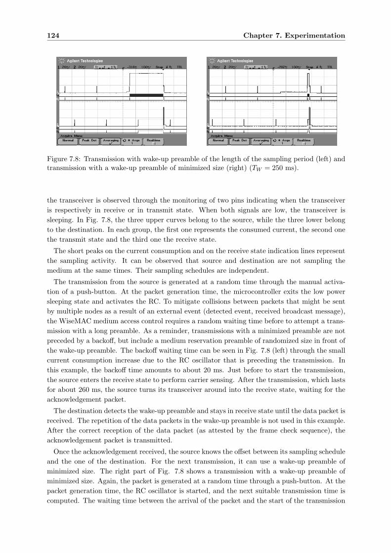
124 Chapter 7. Experimentation
Figure 7.8: Transmission with wake-up preamble of the length of the sampling period (left) andtransmission with a wake-up preamble of minimized size (right) (TW = 250 ms).
the transceiver is observed through the monitoring of two pins indicating when the transceiveris respectively in receive or in transmit state. When both signals are low, the transceiver issleeping. In Fig. 7.8, the three upper curves belong to the source, while the three lower belongto the destination. In each group, the first one represents the consumed current, the second onethe transmit state and the third one the receive state.
The short peaks on the current consumption and on the receive state indication lines representthe sampling activity. It can be observed that source and destination are not sampling themedium at the same times. Their sampling schedules are independent.
The transmission from the source is generated at a random time through the manual activa-tion of a push-button. At the packet generation time, the microcontroller exits the low powersleeping state and activates the RC. To mitigate collisions between packets that might be sentby multiple nodes as a result of an external event (detected event, received broadcast message),the WiseMAC medium access control requires a random waiting time before to attempt a trans-mission with a long preamble. As a reminder, transmissions with a minimized preamble are notpreceded by a backoff, but include a medium reservation preamble of randomized size in front ofthe wake-up preamble. The backoff waiting time can be seen in Fig. 7.8 (left) through the smallcurrent consumption increase due to the RC oscillator that is preceding the transmission. Inthis example, the backoff time amounts to about 20 ms. Just before to start the transmission,the source enters the receive state to perform carrier sensing. After the transmission, which lastsfor about 260 ms, the source turns its transceiver around into the receive state, waiting for theacknowledgement packet.
The destination detects the wake-up preamble and stays in receive state until the data packet isreceived. The repetition of the data packets in the wake-up preamble is not used in this example.After the correct reception of the data packet (as attested by the frame check sequence), theacknowledgement packet is transmitted.
Once the acknowledgement received, the source knows the offset between its sampling scheduleand the one of the destination. For the next transmission, it can use a wake-up preamble ofminimized size. The right part of Fig. 7.8 shows a transmission with a wake-up preamble ofminimized size. Again, the packet is generated at a random time through a push-button. At thepacket generation time, the RC oscillator is started, and the next suitable transmission time iscomputed. The waiting time between the arrival of the packet and the start of the transmission
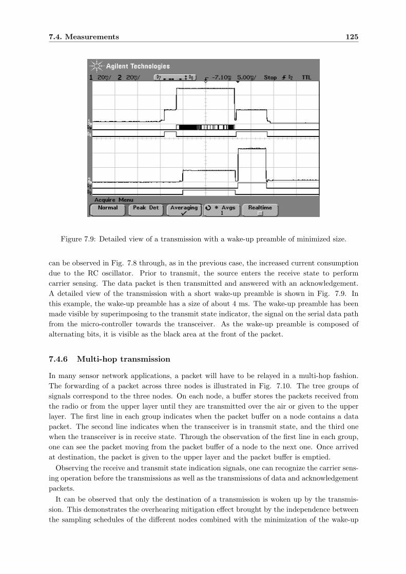
7.4. Measurements 125
Figure 7.9: Detailed view of a transmission with a wake-up preamble of minimized size.
can be observed in Fig. 7.8 through, as in the previous case, the increased current consumptiondue to the RC oscillator. Prior to transmit, the source enters the receive state to performcarrier sensing. The data packet is then transmitted and answered with an acknowledgement.A detailed view of the transmission with a short wake-up preamble is shown in Fig. 7.9. Inthis example, the wake-up preamble has a size of about 4 ms. The wake-up preamble has beenmade visible by superimposing to the transmit state indicator, the signal on the serial data pathfrom the micro-controller towards the transceiver. As the wake-up preamble is composed ofalternating bits, it is visible as the black area at the front of the packet.
7.4.6 Multi-hop transmission
In many sensor network applications, a packet will have to be relayed in a multi-hop fashion.The forwarding of a packet across three nodes is illustrated in Fig. 7.10. The tree groups ofsignals correspond to the three nodes. On each node, a buffer stores the packets received fromthe radio or from the upper layer until they are transmitted over the air or given to the upperlayer. The first line in each group indicates when the packet buffer on a node contains a datapacket. The second line indicates when the transceiver is in transmit state, and the third onewhen the transceiver is in receive state. Through the observation of the first line in each group,one can see the packet moving from the packet buffer of a node to the next one. Once arrivedat destination, the packet is given to the upper layer and the packet buffer is emptied.
Observing the receive and transmit state indication signals, one can recognize the carrier sens-ing operation before the transmissions as well as the transmissions of data and acknowledgementpackets.
It can be observed that only the destination of a transmission is woken up by the transmis-sion. This demonstrates the overhearing mitigation effect brought by the independence betweenthe sampling schedules of the different nodes combined with the minimization of the wake-up
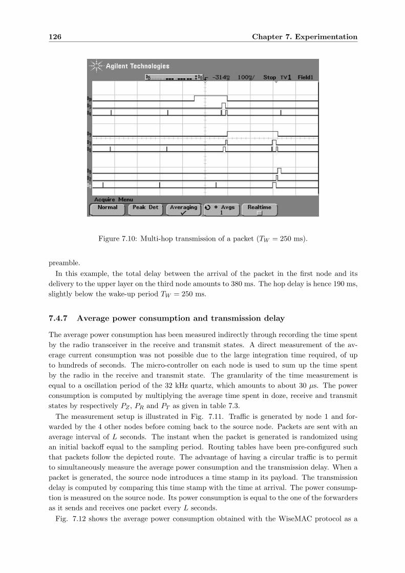
126 Chapter 7. Experimentation
Figure 7.10: Multi-hop transmission of a packet (TW = 250 ms).
preamble.In this example, the total delay between the arrival of the packet in the first node and its
delivery to the upper layer on the third node amounts to 380 ms. The hop delay is hence 190 ms,slightly below the wake-up period TW = 250 ms.
7.4.7 Average power consumption and transmission delay
The average power consumption has been measured indirectly through recording the time spentby the radio transceiver in the receive and transmit states. A direct measurement of the av-erage current consumption was not possible due to the large integration time required, of upto hundreds of seconds. The micro-controller on each node is used to sum up the time spentby the radio in the receive and transmit state. The granularity of the time measurement isequal to a oscillation period of the 32 kHz quartz, which amounts to about 30 µs. The powerconsumption is computed by multiplying the average time spent in doze, receive and transmitstates by respectively PZ , PR and PT as given in table 7.3.
The measurement setup is illustrated in Fig. 7.11. Traffic is generated by node 1 and for-warded by the 4 other nodes before coming back to the source node. Packets are sent with anaverage interval of L seconds. The instant when the packet is generated is randomized usingan initial backoff equal to the sampling period. Routing tables have been pre-configured suchthat packets follow the depicted route. The advantage of having a circular traffic is to permitto simultaneously measure the average power consumption and the transmission delay. When apacket is generated, the source node introduces a time stamp in its payload. The transmissiondelay is computed by comparing this time stamp with the time at arrival. The power consump-tion is measured on the source node. Its power consumption is equal to the one of the forwardersas it sends and receives one packet every L seconds.
Fig. 7.12 shows the average power consumption obtained with the WiseMAC protocol as a
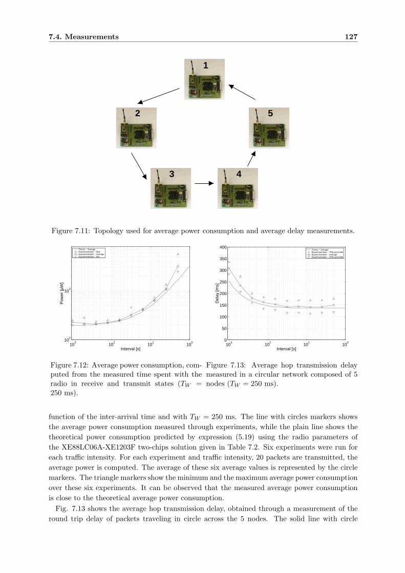
7.4. Measurements 127
1
2
3 4
5
Figure 7.11: Topology used for average power consumption and average delay measurements.
100
101
102
103
102
103
Interval [s]
Pow
er [µ
W]
Theory − AverageExperimentation − MaxExperimentation − AverageExperimentation − Min
Figure 7.12: Average power consumption, com-puted from the measured time spent with theradio in receive and transmit states (TW =250 ms).
100
101
102
103
0
50
100
150
200
250
300
350
400
Interval [s]
Del
ay [m
s]
Theory − AverageExperimentation − 75th percentileExperimentation − AverageExperimentation − 25th percentile
Figure 7.13: Average hop transmission delaymeasured in a circular network composed of 5nodes (TW = 250 ms).
function of the inter-arrival time and with TW = 250 ms. The line with circles markers showsthe average power consumption measured through experiments, while the plain line shows thetheoretical power consumption predicted by expression (5.19) using the radio parameters ofthe XE88LC06A-XE1203F two-chips solution given in Table 7.2. Six experiments were run foreach traffic intensity. For each experiment and traffic intensity, 20 packets are transmitted, theaverage power is computed. The average of these six average values is represented by the circlemarkers. The triangle markers show the minimum and the maximum average power consumptionover these six experiments. It can be observed that the measured average power consumptionis close to the theoretical average power consumption.
Fig. 7.13 shows the average hop transmission delay, obtained through a measurement of theround trip delay of packets traveling in circle across the 5 nodes. The solid line with circle
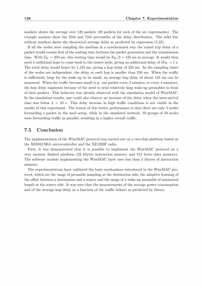
128 Chapter 7. Experimentation
markers shows the average over 120 packets (20 packets for each of the six experiments). Thetriangle markers show the 25th and 75th percentiles of the delay distribution. The solid linewithout markers shows the theoretical average delay as predicted by expression (5.23).
If all the nodes were sampling the medium in a synchronized way the round trip delay of apacket would consist first of the waiting time between the packet generation and the transmissiontime. With TW = 250 ms, this waiting time would be TW /2 = 125 ms in average. It would thenneed 4 additional hops to come back to the source node, giving an additional delay of 4TW = 1 s.The total delay would hence be 1.125 ms, giving a hop delay of 225 ms. As the sampling timesof the nodes are independent, the delay at each hop is smaller than 250 ms. When the trafficis sufficiently large for the wake-up to be small, an average hop delay of about 125 ms can bemeasured. When the traffic becomes small (e.g. one packet every 2 minutes, or every 4 minutes),the hop delay augments because of the need to send relatively long wake-up preambles in frontof data packets. This behavior was already observed with the simulation model of WiseMAC.In the simulation results, one could also observe an increase of the delay when the inter-arrivaltime was below L = 10 s. This delay increase in high traffic conditions is not visible in theresults of this experiment. The reason of this better performance is that there are only 5 nodesforwarding a packet in the used setup, while in the simulated network, 10 groups of 10 nodeswere forwarding traffic in parallel, resulting in a higher overall traffic.
7.5 Conclusion
The implementation of the WiseMAC protocol was carried out on a two-chip platform based onthe XE88LC06A microcontroller and the XE1203F radio.
First, it was demonstrated that it is possible to implement the WiseMAC protocol on avery memory limited platform (22 kbytes instruction memory and 512 bytes data memory).The software module implementing the WiseMAC layer uses less than 5 kbytes of instructionmemory.
The experimentations have validated the basic mechanisms introduced in the WiseMAC pro-tocol, which are the usage of preamble sampling at the destination side, the adaptive learning ofthe offset between a destination and a source and the usage of a wake-up preamble of minimizedlength at the source side. It was seen that the measurements of the average power consumptionand of the average hop delay as a function of the traffic behave as predicted by theory.
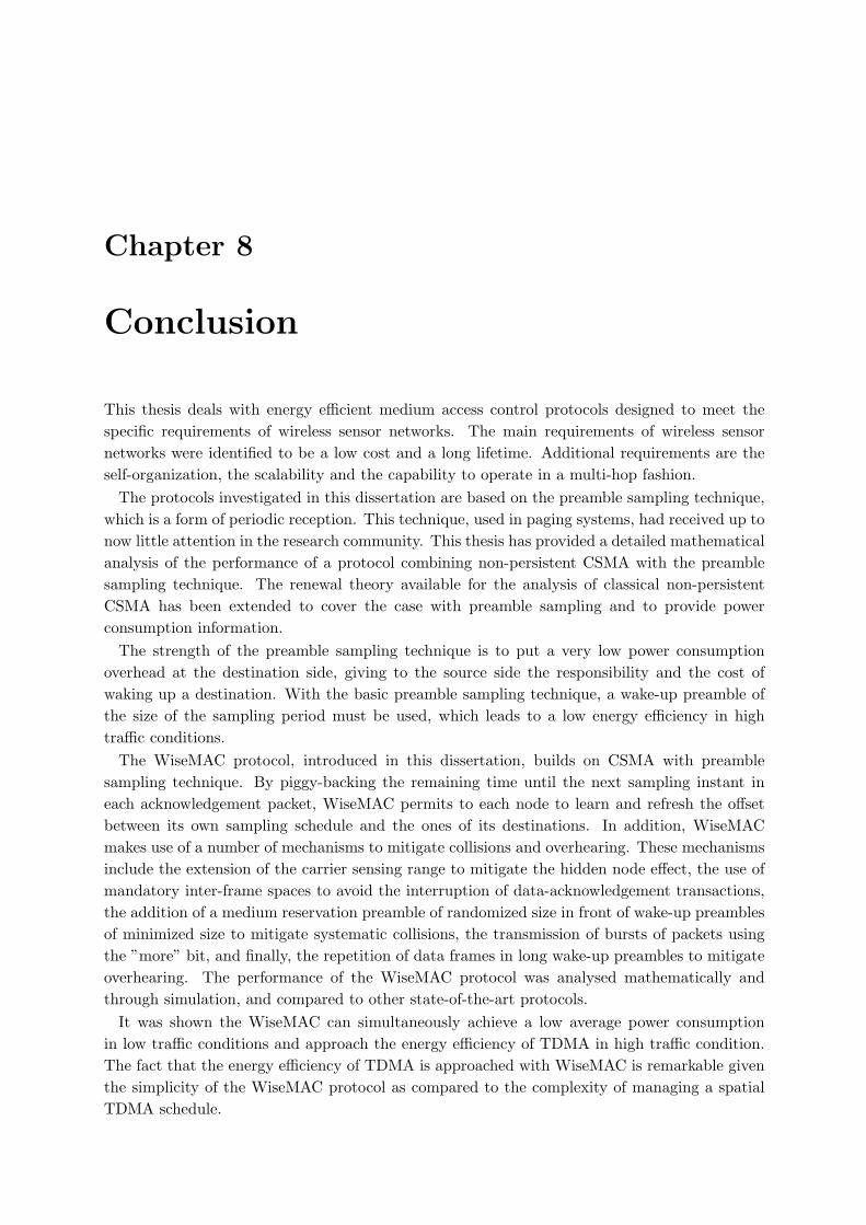
Chapter 8
Conclusion
This thesis deals with energy efficient medium access control protocols designed to meet thespecific requirements of wireless sensor networks. The main requirements of wireless sensornetworks were identified to be a low cost and a long lifetime. Additional requirements are theself-organization, the scalability and the capability to operate in a multi-hop fashion.
The protocols investigated in this dissertation are based on the preamble sampling technique,which is a form of periodic reception. This technique, used in paging systems, had received up tonow little attention in the research community. This thesis has provided a detailed mathematicalanalysis of the performance of a protocol combining non-persistent CSMA with the preamblesampling technique. The renewal theory available for the analysis of classical non-persistentCSMA has been extended to cover the case with preamble sampling and to provide powerconsumption information.
The strength of the preamble sampling technique is to put a very low power consumptionoverhead at the destination side, giving to the source side the responsibility and the cost ofwaking up a destination. With the basic preamble sampling technique, a wake-up preamble ofthe size of the sampling period must be used, which leads to a low energy efficiency in hightraffic conditions.
The WiseMAC protocol, introduced in this dissertation, builds on CSMA with preamblesampling technique. By piggy-backing the remaining time until the next sampling instant ineach acknowledgement packet, WiseMAC permits to each node to learn and refresh the offsetbetween its own sampling schedule and the ones of its destinations. In addition, WiseMACmakes use of a number of mechanisms to mitigate collisions and overhearing. These mechanismsinclude the extension of the carrier sensing range to mitigate the hidden node effect, the use ofmandatory inter-frame spaces to avoid the interruption of data-acknowledgement transactions,the addition of a medium reservation preamble of randomized size in front of wake-up preamblesof minimized size to mitigate systematic collisions, the transmission of bursts of packets usingthe ”more” bit, and finally, the repetition of data frames in long wake-up preambles to mitigateoverhearing. The performance of the WiseMAC protocol was analysed mathematically andthrough simulation, and compared to other state-of-the-art protocols.
It was shown the WiseMAC can simultaneously achieve a low average power consumptionin low traffic conditions and approach the energy efficiency of TDMA in high traffic condition.The fact that the energy efficiency of TDMA is approached with WiseMAC is remarkable giventhe simplicity of the WiseMAC protocol as compared to the complexity of managing a spatialTDMA schedule.
130 Chapter 8. Conclusion
When using the WiseNET SoC, a node will consume only 28 µW to forward a packet of 60bytes every 100 seconds. A lifetime of 5 years could then be reached using a single AA alkalinebattery. The WiseMAC protocol was shown, at that traffic, to be 75 times more energy efficientthan the classical non-power saving CSMA/CA and 8 times better than S-MAC, operated at itsdefault duty cycle of 10%.
An implementation of the WiseMAC protocol on a low-power embedded platform has demon-strated the practical validity of the proposed mechanisms. It was shown that this protocol canbe implemented with a memory footprint of a few kbytes only, as required to meet the low costrequirement. Measurements of the average power consumption and of the average hop delayhave confirmed results provided by the mathematical analysis and by simulations.
The WiseMAC protocol was shown to be an attractive MAC protocol, not only for wirelessmulti-hop sensor network, but also for the downlink of infrastructured based wireless sensornetworks, allowing the use of a single scheme for communication in a hybrid topology.
The WiseMAC protocol was designed to operate on a single frequency. A direction for furtherdevelopment could be to target the support of multiple frequency channels, in order to increasethe system capacity and be able to avoid interferers through frequency agility.
At the physical layer, further work will be needed to evaluate the trade-offs between the usedbit rate, the transmission power, the modulation and the channel coding schemes in the contextof low duty cycle wireless sensor networks.
At the network layer, further work include the evaluation of routing protocols suitable foroperating above the WiseMAC layer. The WiseMAC protocol is based on a flat topology,as opposed to a clustered topology with for example the IEEE 802.15.4 protocol [82]. Thischaracteristic may help in designing simple routing algorithms. With WiseMAC, broadcasttransmissions must be of the duration of the sampling period to wake up and reach every nodein range. Broadcast is used by many multi-hop routing protocols such as DSR [51] or directeddiffusion [49]. As using long wake-up preambles is energetically costly, the usage of broadcastswill negatively impact power consumption. The support of mobility will require broadcastmessages for network discovery. A high mobility will be associated with a relatively high powerconsumption. However, many sensor network applications are expected to be quasi static. Insuch cases, the energetic cost of self-organization can be expected to be low. When mobilityis desired, solutions to implement an energy efficient routing on top of the WiseMAC protocolremain to be designed.
Congestion is a source of collisions and energy waste. Flow control is traditionally implementedbetween end-points at the transport layer. In a multi-hop sensor network, it may be of interest,as proposed by Woo in [122], to insert a ”stop” bit in the MAC layer acknowledgements. Such amechanism is compatible with the WiseMAC protocol. Its performances remain to be evaluatedin conjunction to WiseMAC. This scheme may permit to inform more rapidly the sources of acongestion than classical transport layer schemes.
A further potential source of energy savings can be found in the field of mobile code. Mobilecode may save energy, for example, in applications where distributed processing would requiremore energy to transfer the information to be processed than to transfer the algorithm to beapplied to the data.
Appendix A
Interference Between Bluetooth
Piconets
A.1 Introduction
Bluetooth is a digital wireless data transmission standard in the 2.4 GHz ISM band aimed atproviding a short range wireless link between laptops, cellular phones and other devices [102].The air interface modulation is Gaussian FSK with a raw bit rate of 1 Mb/s. The communicationtopology between Bluetooth nodes is point-to-multipoint, where a master communicates in timedivision duplex with several slaves forming a so-called piconet. Even slots are used for packetsfrom the master to one of the slaves and odd slots are used for the return direction. In orderto tolerate interference which can readily arise in the 2.4 GHz band, a slow frequency hoppingscheme is used, where all nodes of a piconet hop together among 79 frequencies at each packetslot. As Bluetooth is meant to be used for applications such as connecting a headset to a mobilephone, the problem of co-channel interference from other Bluetooth piconets can become of highimportance. It is likely to have several persons in proximity, each having an open Bluetoothconnection between a mobile phone and a headset or a mobile computer. Simulation resultsaddressing the problem of interference between Bluetooth networks can also be found in [137]and [136].
A.2 Model
We assume n unsynchronized collocated piconets that are sufficiently close from one another suchthat a co-channel interference between 2 or more packets will destroy all packets. For simplicity,we assume that only 1 bit of overlap is enough to destroy all packets involved. The interferencesystem model is shown in Fig. 1. Forward error correction and capture effect are neglected.Because of the strong adjacent channel rejection requirement imposed by the standard, adjacentchannel interference is not considered. The traffic in each piconet is assumed periodic and thepacket rate is G packets per slot. G can take values between 0 and 1 and can be seen as theprobability to have a packet in a slot. With G = 1, we have 100% traffic in each piconet.
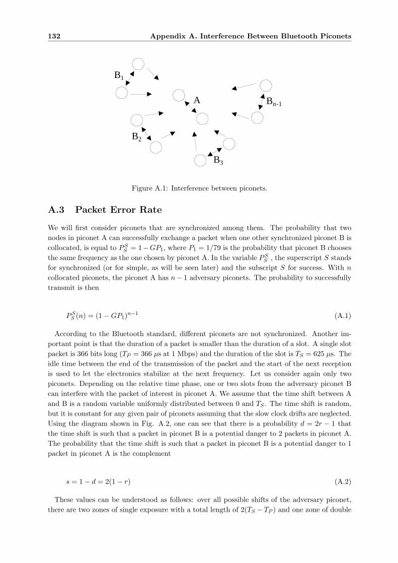
132 Appendix A. Interference Between Bluetooth Piconets
A
B1
B2
B3
Bn-1
Figure A.1: Interference between piconets.
A.3 Packet Error Rate
We will first consider piconets that are synchronized among them. The probability that twonodes in piconet A can successfully exchange a packet when one other synchronized piconet B iscollocated, is equal to PS
S = 1−GP1, where P1 = 1/79 is the probability that piconet B choosesthe same frequency as the one chosen by piconet A. In the variable PS
S , the superscript S standsfor synchronized (or for simple, as will be seen later) and the subscript S for success. With n
collocated piconets, the piconet A has n− 1 adversary piconets. The probability to successfullytransmit is then
PSS (n) = (1−GP1)n−1 (A.1)
According to the Bluetooth standard, different piconets are not synchronized. Another im-portant point is that the duration of a packet is smaller than the duration of a slot. A single slotpacket is 366 bits long (TP = 366 µs at 1 Mbps) and the duration of the slot is TS = 625 µs. Theidle time between the end of the transmission of the packet and the start of the next receptionis used to let the electronics stabilize at the next frequency. Let us consider again only twopiconets. Depending on the relative time phase, one or two slots from the adversary piconet Bcan interfere with the packet of interest in piconet A. We assume that the time shift between Aand B is a random variable uniformly distributed between 0 and TS . The time shift is random,but it is constant for any given pair of piconets assuming that the slow clock drifts are neglected.Using the diagram shown in Fig. A.2, one can see that there is a probability d = 2r − 1 thatthe time shift is such that a packet in piconet B is a potential danger to 2 packets in piconet A.The probability that the time shift is such that a packet in piconet B is a potential danger to 1packet in piconet A is the complement
s = 1− d = 2(1− r) (A.2)
These values can be understood as follows: over all possible shifts of the adversary piconet,there are two zones of single exposure with a total length of 2(TS − TP ) and one zone of double
A.3. Packet Error Rate 133
TS
Piconet A
Piconet B
TP TS TP-
Singlevulnerability
Doublevulnerability
Singlevulnerability
Figure A.2: Single or double exposition to interference.
exposure of length TP − (TS − TP ) = 2TP − TS . Normalized with TS and using r = TP /TS , weobtain 2(1− r) and 2r − 1.
If the adversary piconet B is shifted such that one of its packets is threatening two slots inpiconet A, the probability of transmitting successfully one packet is given by PD
S = (1−GP1)2,as both the preceding and the following slots must have chosen another frequency, in the casethat they had a packet to send1. In the variable PD
S , D stands for double exposure. Now, ifthere are n collocated piconets, and if all n − 1 adversary piconets are shifted such that eachof the packet sent by them is doubly threatening a packet sent in piconet A, the probability tosuccessfully transmit becomes
PDS (n) = (1−GP1)2(n−1) (A.3)
In a real situation, from the n− 1 adversary piconets, there will be a number nS of piconetssimply threatening and a number nD = n − 1 − nS of piconets doubly threatening. Thesenumbers are random but constant over time for any given set of active piconets. Let denotewith NS the random variable taking individual values nS . The distribution of NS is binomial:
P(NS = ns) =(
n− 1nS
)snS (1− s)n−1−nS (A.4)
where s is defined in equation (A.2). For any given n and nS , the probability of successfullytransmitting a packet can be expressed as
1Another way to see this is to consider that the packet will suffer from interference and be in error if bothdangerous slots choose the same frequency and have a packet to send (probability (GP1)
2), or if the first onechooses the same frequency and have a packet to send and the second doesn’t (probability GP1(1−GP1)). Thislast event can be reversed. Therefore, the probability to have a packet error is P D
E = 2GP1(1−GP1) + (GP1)2 =
2GP1 − (GP1)2 and P D
S = 1− P DE = (1−GP1)
2.
134 Appendix A. Interference Between Bluetooth Piconets
PS(n, nS) = (1−GP1)nS (1−GP1)2(n−1−nS) = (1−GP1)2(n−1)−ns (A.5)
This expression is a lower bound on the packet success probability as a function of n and nS .The packet success probability can be higher in a real system thanks to the capture effect andforward error correction codes. With ns = n− 1 , we obtain the synchronized case, i.e. formula(A.1). With nS = 0, we obtain the double threat case, i.e. formula (A.3). The mean value ofthis lower bound over all possible shift configurations can be obtained by taking the expectationof (A.5) over all values of NS :
PS(n) = E [PS(n, NS)]
=n−1∑
nS=0(1−GP1)
nS (1−GP1)2(n−1−nS)
(n− 1nS
)snS (1− s)n−1−nS
=n−1∑
nS=0
(n− 1nS
)(s (1−GP1))
nS
((1− s) (1−GP1)
2)n−1−nS
=(s (1−GP1) + (1− s) (1−GP1)
2)n−1
where we made use of the expansion formula for the Newton’s binomial
(x + y)n =n∑
k=0
(n
k
)xkyn−k
Replacing the variable s by TP /TS , we get
PS(n) =(
2(
1− TP
TS
)(1−GP1) +
(2TP
TS− 1
)(1−GP1)
2
)n−1
(A.6)
A simpler way to find the same result, valid when G = 1, is given in [24]. Defining aM =s (1−GP1) + (1− s) (1−GP1)
2, we obtain PS(n) = an−1M , where M stands for mean. We see
that in the three considered scenarios, the expression for the packet success probability has theform
PS(n) = an−1 (A.7)
where a depends on the scenario. In the one considered at last, for G = 1, we have a = aM =s (1− P1)+(1− s) (1− P1)
2 = 0.9852. If we would have considered unsynchronized piconets butwould not have taken into account the fact that the packet length is smaller than the slot length,we would be in the situation where nD = n−1 , with a = aD = (1−P1)2 = (1−1/79)2 = 0.9748.This corresponds to aM with s = 0. With synchronized piconets, the ratio between packet andslot length is not relevant. We have always only one dangerous slot in an adversary piconet.The value of the variable a is then a = aS = 1 − P1 = 1 − 1/79 = 0.9873. This corresponds toaM with s = 1. Assuming n unsynchronized piconets all transmitting with a packet rate G = 1,the packet error rate suffered by one piconet because of the interference from n − 1 adversary
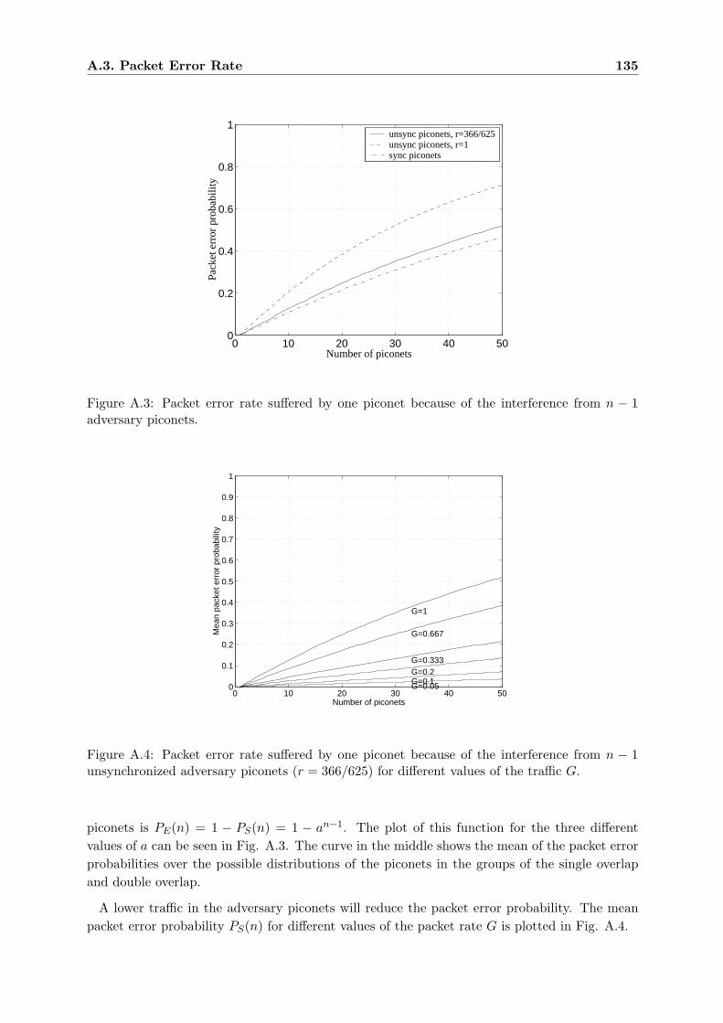
A.3. Packet Error Rate 135
0 10 20 30 40 500
0.2
0.4
0.6
0.8
1
Number of piconets
Pack
et e
rror
pro
babi
lity
unsync piconets, r=366/625unsync piconets, r=1sync piconets
Figure A.3: Packet error rate suffered by one piconet because of the interference from n − 1adversary piconets.
0 10 20 30 40 500
0.1
0.2
0.3
0.4
0.5
0.6
0.7
0.8
0.9
1
G=0.05G=0.1G=0.2G=0.333
G=0.667
G=1
Number of piconets
Mea
n pa
cket
err
or p
roba
bilit
y
Figure A.4: Packet error rate suffered by one piconet because of the interference from n − 1unsynchronized adversary piconets (r = 366/625) for different values of the traffic G.
piconets is PE(n) = 1 − PS(n) = 1 − an−1. The plot of this function for the three differentvalues of a can be seen in Fig. A.3. The curve in the middle shows the mean of the packet errorprobabilities over the possible distributions of the piconets in the groups of the single overlapand double overlap.
A lower traffic in the adversary piconets will reduce the packet error probability. The meanpacket error probability PS(n) for different values of the packet rate G is plotted in Fig. A.4.
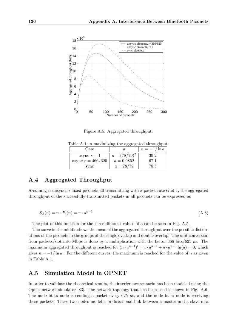
136 Appendix A. Interference Between Bluetooth Piconets
0 50 100 150 200 250 3000
2
4
6
8
10
12
14
16
18x 10
6
Number of piconets
Agg
rega
ted
thro
ughp
ut [
bit/s
]
unsync piconets, r=366/625unsync piconets, r=1sync piconets
Figure A.5: Aggregated throughput.
Table A.1: n maximizing the aggregated throughput.Case a n = −1/ ln a
async r = 1 a = (78/79)2 39.2async r = 466/625 a = 0.9852 67.1
sync a = 78/79 78.5
A.4 Aggregated Throughput
Assuming n unsynchronized piconets all transmitting with a packet rate G of 1, the aggregatedthroughput of the successfully transmitted packets in all piconets can be expressed as
SA(n) = n · Ps(n) = n · an−1 (A.8)
The plot of this function for the three different values of a can be seen in Fig. A.5.The curve in the middle shows the mean of the aggregated throughput over the possible distrib-
utions of the piconets in the groups of the single overlap and double overlap. The unit conversionfrom packets/slot into Mbps is done by a multiplication with the factor 366 bits/625 µs. Themaximum aggregated throughput is reached for (n · an−1)′ = 1 · an−1 + n · an−1 ln(a) = 0, whichgives n = −1/ ln a . For the different curves, the maximum is reached for the value of n as givenin Table A.1.
A.5 Simulation Model in OPNET
In order to validate the theoretical results, the interference scenario has been modeled using theOpnet network simulator [83]. The network topology that has been used is shown in Fig. A.6.The node bt tx node is sending a packet every 625 µs, and the node bt rx node is receivingthese packets. These two nodes model a bi-directional link between a master and a slave in a
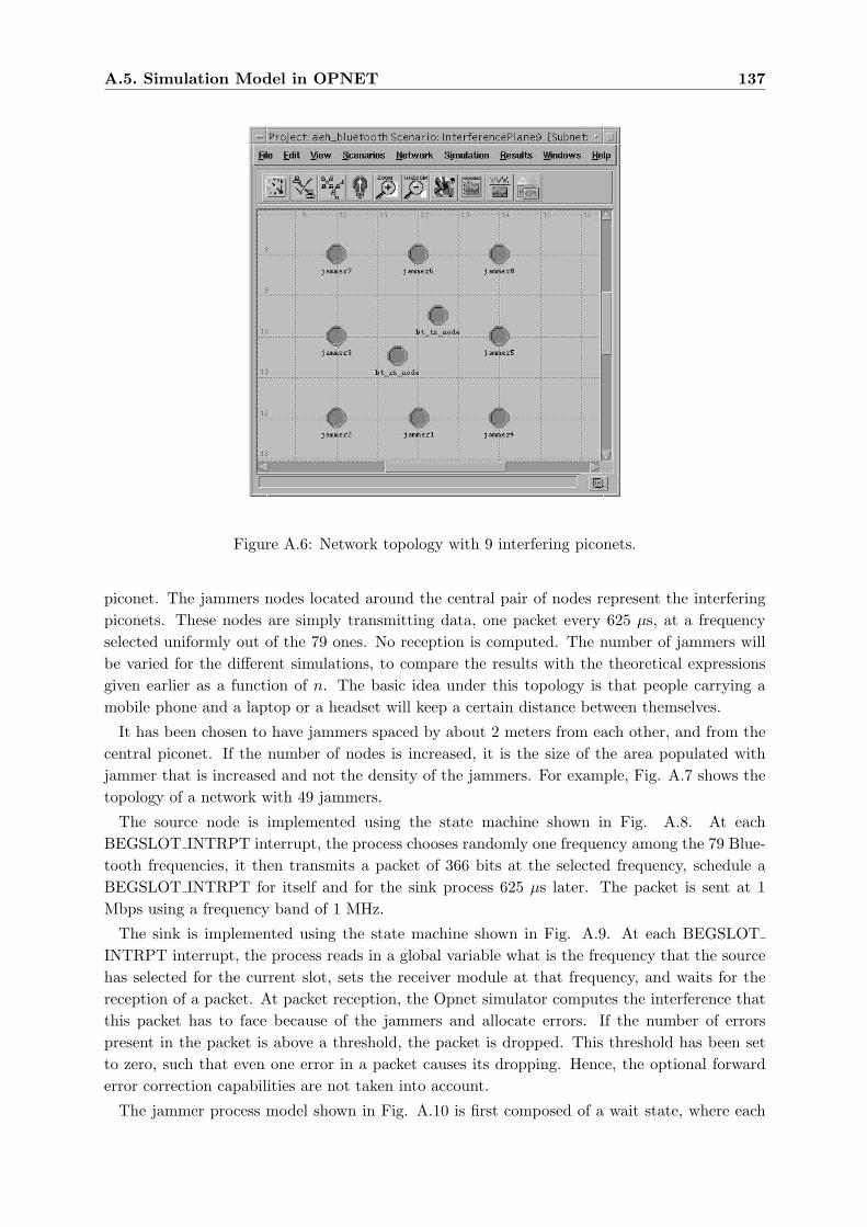
A.5. Simulation Model in OPNET 137
Figure A.6: Network topology with 9 interfering piconets.
piconet. The jammers nodes located around the central pair of nodes represent the interferingpiconets. These nodes are simply transmitting data, one packet every 625 µs, at a frequencyselected uniformly out of the 79 ones. No reception is computed. The number of jammers willbe varied for the different simulations, to compare the results with the theoretical expressionsgiven earlier as a function of n. The basic idea under this topology is that people carrying amobile phone and a laptop or a headset will keep a certain distance between themselves.
It has been chosen to have jammers spaced by about 2 meters from each other, and from thecentral piconet. If the number of nodes is increased, it is the size of the area populated withjammer that is increased and not the density of the jammers. For example, Fig. A.7 shows thetopology of a network with 49 jammers.
The source node is implemented using the state machine shown in Fig. A.8. At eachBEGSLOT INTRPT interrupt, the process chooses randomly one frequency among the 79 Blue-tooth frequencies, it then transmits a packet of 366 bits at the selected frequency, schedule aBEGSLOT INTRPT for itself and for the sink process 625 µs later. The packet is sent at 1Mbps using a frequency band of 1 MHz.
The sink is implemented using the state machine shown in Fig. A.9. At each BEGSLOTINTRPT interrupt, the process reads in a global variable what is the frequency that the sourcehas selected for the current slot, sets the receiver module at that frequency, and waits for thereception of a packet. At packet reception, the Opnet simulator computes the interference thatthis packet has to face because of the jammers and allocate errors. If the number of errorspresent in the packet is above a threshold, the packet is dropped. This threshold has been setto zero, such that even one error in a packet causes its dropping. Hence, the optional forwarderror correction capabilities are not taken into account.
The jammer process model shown in Fig. A.10 is first composed of a wait state, where each
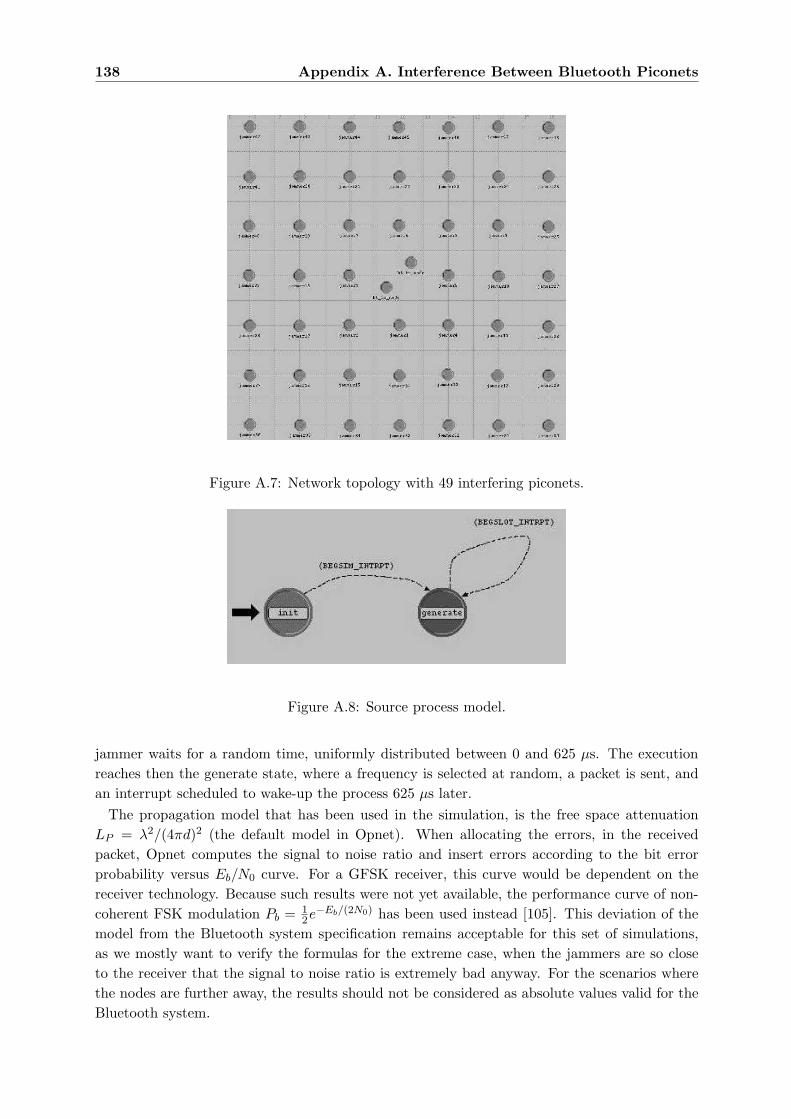
138 Appendix A. Interference Between Bluetooth Piconets
Figure A.7: Network topology with 49 interfering piconets.
Figure A.8: Source process model.
jammer waits for a random time, uniformly distributed between 0 and 625 µs. The executionreaches then the generate state, where a frequency is selected at random, a packet is sent, andan interrupt scheduled to wake-up the process 625 µs later.
The propagation model that has been used in the simulation, is the free space attenuationLP = λ2/(4πd)2 (the default model in Opnet). When allocating the errors, in the receivedpacket, Opnet computes the signal to noise ratio and insert errors according to the bit errorprobability versus Eb/N0 curve. For a GFSK receiver, this curve would be dependent on thereceiver technology. Because such results were not yet available, the performance curve of non-coherent FSK modulation Pb = 1
2e−Eb/(2N0) has been used instead [105]. This deviation of themodel from the Bluetooth system specification remains acceptable for this set of simulations,as we mostly want to verify the formulas for the extreme case, when the jammers are so closeto the receiver that the signal to noise ratio is extremely bad anyway. For the scenarios wherethe nodes are further away, the results should not be considered as absolute values valid for theBluetooth system.
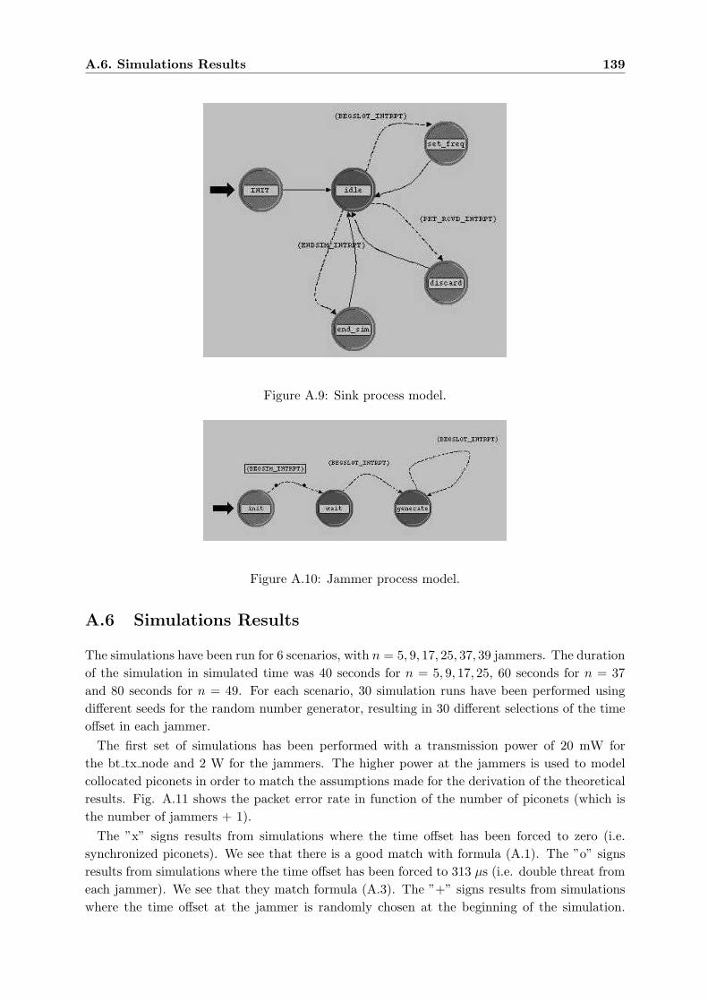
A.6. Simulations Results 139
Figure A.9: Sink process model.
Figure A.10: Jammer process model.
A.6 Simulations Results
The simulations have been run for 6 scenarios, with n = 5, 9, 17, 25, 37, 39 jammers. The durationof the simulation in simulated time was 40 seconds for n = 5, 9, 17, 25, 60 seconds for n = 37and 80 seconds for n = 49. For each scenario, 30 simulation runs have been performed usingdifferent seeds for the random number generator, resulting in 30 different selections of the timeoffset in each jammer.
The first set of simulations has been performed with a transmission power of 20 mW forthe bt tx node and 2 W for the jammers. The higher power at the jammers is used to modelcollocated piconets in order to match the assumptions made for the derivation of the theoreticalresults. Fig. A.11 shows the packet error rate in function of the number of piconets (which isthe number of jammers + 1).
The ”x” signs results from simulations where the time offset has been forced to zero (i.e.synchronized piconets). We see that there is a good match with formula (A.1). The ”o” signsresults from simulations where the time offset has been forced to 313 µs (i.e. double threat fromeach jammer). We see that they match formula (A.3). The ”+” signs results from simulationswhere the time offset at the jammer is randomly chosen at the beginning of the simulation.
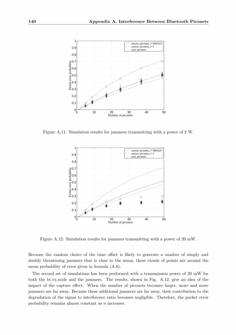
140 Appendix A. Interference Between Bluetooth Piconets
0 10 20 30 40 500
0.1
0.2
0.3
0.4
0.5
0.6
0.7
0.8
0.9
1
Number of piconets
Pack
et e
rror
pro
babi
lity
unsync piconets, r=366/625unsync piconets, r=1sync piconets
Figure A.11: Simulation results for jammers transmitting with a power of 2 W.
0 10 20 30 40 500
0.1
0.2
0.3
0.4
0.5
0.6
0.7
0.8
0.9
1
Number of piconets
Pack
et e
rror
pro
babi
lity
unsync piconets, r=366/625unsync piconets, r=1sync piconets
Figure A.12: Simulation results for jammers transmitting with a power of 20 mW.
Because the random choice of the time offset is likely to generate a number of simply anddoubly threatening jammers that is close to the mean, these clouds of points are around themean probability of error given in formula (A.6).
The second set of simulations has been performed with a transmission power of 20 mW forboth the bt tx node and the jammers. The results, shown in Fig. A.12, give an idea of theimpact of the capture effect. When the number of piconets becomes larger, more and morejammers are far away. Because these additional jammers are far away, their contribution to thedegradation of the signal to interference ratio becomes negligible. Therefore, the packet errorprobability remains almost constant as n increases.
A.7. Conclusion 141
A.7 Conclusion
The analysis presented here gives an upper bound on the mean packet error rate of a Bluetoothlink under co-channel interference from n − 1 other piconets, as well as a lower bound on theaggregated throughput of n collocated piconets. In a more general way, this analysis providessome insights to the problem of co-channel interference between Bluetooth piconets. It permitsalso to quantify the potential gain that one would obtain if different piconets would be synchro-nized by some means external to the Bluetooth standard. These expressions, as they do nottake into account the effect of capture and the possible correction of errors using forward errorcorrection, can be used to measure these effects in terms of packet error probability reduction.Simulation results illustrate this probabilistic analysis and show the potential effect of captureon the packet error probability.

Appendix B
Simulation Model
B.1 Simulation plateform
Because of the complex nature of multi-hop wireless sensor networks, there is a strong need toperform simulations of newly designed communication protocols, before to attempt implemen-tation and real world testing.
At the time of the project start (in 2001), there existed only few discrete event networksimulators that could be used for wireless MAC protocol simulation1: OPNET [83], NS-2 [113]and Glomosim [134].
OPNET is a very popular commercial tool, where protocols are implemented in pseudo-Clanguage inside finite state machines. NS-2 is widely used among routing and transport protocolsresearchers, mainly in the field of TCP/IP wired networks. A wireless component has been addedto enable research on adaptive routing for wireless ad hoc networks. Protocols are implementedin C++ and simulations scenarios are defined with Object Tcl scripts. Glomosim is a simulatordedicated to the simulation of wireless networks. It aims at providing a short execution time ofsimulation involving tens of wireless nodes. Glomosim has been developed on top of the discreteevent simulation language ”Parsec”. This language is composed of a very limited number ofcommands (mainly send, send after some delay and hold). The core of the software is thescheduler, which is passing messages among nodes and continuously reordering the list of futureevents. Building upon simple constructs, the Glomosim software has evolved towards a complexsimulator offering an OSI layered structure, with a number of different ad hoc routing andwireless medium access control protocols. Because of its processing efficiency, its clean softwarestructure and its open source character, we have decided to use and extend this simulator.Another advantage of Glomosim is that it is written in C, a language that is likely to be used forimplementations on embedded sensors, thereby allowing a potential reuse of parts of the MAClayer model source code for the implementation.
B.2 Interference and radio layer simulation model
The radio layer of Glomosim did not include the modeling of low power functions. This modelhad to be completed with the addition of a doze state, where packets cannot be received, as
1Newly developed simulation platforms include SENSE [108] and JiST/SWANS [5]. Note that Glomosimhas evolved into the commercial QualNET simulator [97]. The open source Glomosim simulator has not beendeveloped any further since year 2000.
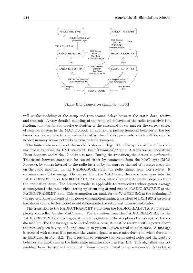
144 Appendix B. Simulation Model
RADIO_DOZE
MAC Request Setup RX/Start Timer Setup RX
RADIO_SET UP_RX RADIO_SETUP_TX
RADIO_READY_RX RADIO_READY_TX
RADIO_TRANSMITRADIO_RECEIVE
MAC Request Setup TX/Start Timer Setup TX
TimerTimer
Start of msg [SNR ok]
End of msg [SNR sill ok]/give to MAC layer MAC Request
Start TX/Start Timer
Message Duration
Timer
MAC Request/Doze
MAC Request/Doze
MAC RequestSetup TX/Start Timer
Turn around RX-TX
MAC RequestSetup RX/Start Timer
Turn around TX-RX
Figure B.1: Transceiver simulation model
well as the modeling of the setup and turn-around delays between the states doze, receiveand transmit. A very detailed modeling of the temporal behavior of the radio transceiver is afundamental step for the precise evaluation of the consumed power and for the correct choiceof time parameters in the MAC protocol. In addition, a precise temporal behavior of the lowlayers is a prerequisite to any evaluation of synchronization protocols, which will for sure beneeded in many sensor networks to provide time stamping.
The finite state machine of the model is shown in Fig. B.1. The syntax of the finite statemachine is following the UML standard: Event [Condition]/Action. A transition is made if theEvent happens and if the Condition is met. During the transition, the Action is performed.Transitions between states can be caused either by commands from the MAC layer (MACRequest), by timers internal to the radio layer or by the start or the end of message receptionon the radio medium. In the RADIO DOZE state, the radio cannot send, nor receive. Itconsumes very little energy. On request from the MAC layer, the radio layer goes into theRADIO READY TX or RADIO READY RX states, after a waiting delay that depends fromthe originating state. The designed model is applicable to transceivers whose power averageconsumption is the same when setting up or turning around into the RADIO RECEIVE or theRADIO TRANSMIT state. This assumption was made for the WiseNET SoC at the beginning ofthe project. Measurements of the power consumption during transitions of a XE1203 transceiverhas shown that a better model would differentiate the setup and turn-around states.
The transition to the RADIO TRANSMIT state from the RADIO READY TX state is com-pletely controlled by the MAC layer. The transition from the RADIO READY RX to theRADIO RECEIVE state is triggered by the beginning of the reception of a message on the ra-dio medium. For the message to be locked with success, it must be received with a power abovethe receiver’s sensitivity, and large enough to present a given signal to noise ratio. A messageis received with success if it presents the wanted signal to noise ratio during its whole duration,as illustrated in Fig. B.2. The algorithm to compute the accumulated noise and the capturebehavior are illustrated in the finite state machine shown in Fig. B.3. This algorithm was notmodified from the one in the original Glomosim accumulated noise radio model: A packet is
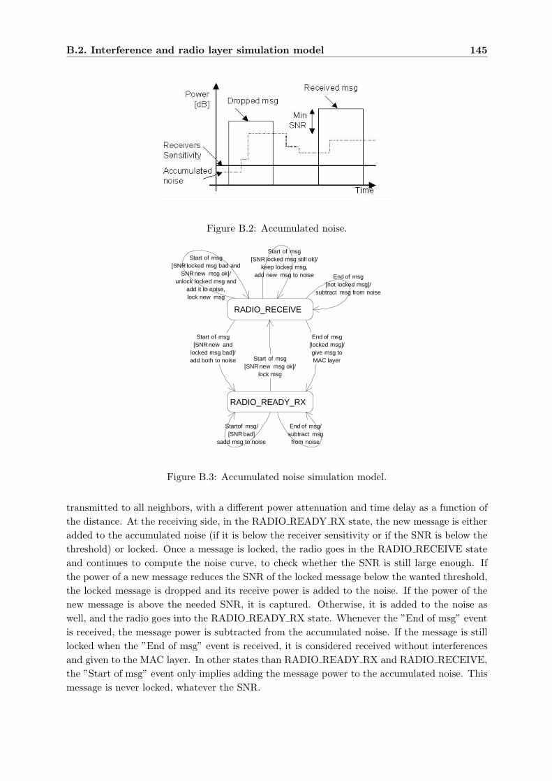
B.2. Interference and radio layer simulation model 145
Figure B.2: Accumulated noise.
RADIO_READY_RX
RADIO_RECEIVE
Start of msg[SNR new msg ok]/
lock msg
End of msg[locked msg]/give msg toMAC layer
Start of msg[SNR locked msg bad and
SNR new msg ok]/unlock locked msg and
add it to noise,lock new msg
Start of msg[SNR locked msg still ok]/
keep locked msg,add new msg to noise End of msg
[not locked msg]/subtract msg from noise
Start of msg[SNR new and
locked msg bad]/add both to noise
End of msg/subtract msg
from noise
Startof msg/[SNR bad]
sadd msg to noise
Figure B.3: Accumulated noise simulation model.
transmitted to all neighbors, with a different power attenuation and time delay as a function ofthe distance. At the receiving side, in the RADIO READY RX state, the new message is eitheradded to the accumulated noise (if it is below the receiver sensitivity or if the SNR is below thethreshold) or locked. Once a message is locked, the radio goes in the RADIO RECEIVE stateand continues to compute the noise curve, to check whether the SNR is still large enough. Ifthe power of a new message reduces the SNR of the locked message below the wanted threshold,the locked message is dropped and its receive power is added to the noise. If the power of thenew message is above the needed SNR, it is captured. Otherwise, it is added to the noise aswell, and the radio goes into the RADIO READY RX state. Whenever the ”End of msg” eventis received, the message power is subtracted from the accumulated noise. If the message is stilllocked when the ”End of msg” event is received, it is considered received without interferencesand given to the MAC layer. In other states than RADIO READY RX and RADIO RECEIVE,the ”Start of msg” event only implies adding the message power to the accumulated noise. Thismessage is never locked, whatever the SNR.

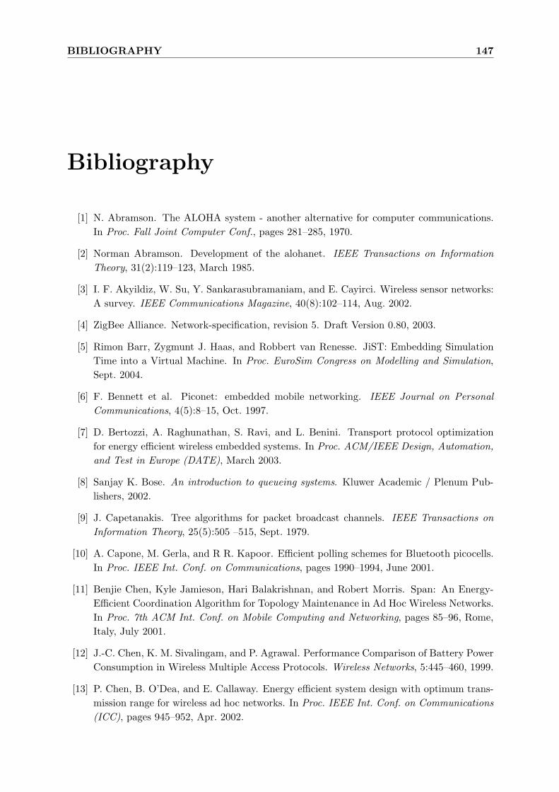
BIBLIOGRAPHY 147
Bibliography
[1] N. Abramson. The ALOHA system - another alternative for computer communications.In Proc. Fall Joint Computer Conf., pages 281–285, 1970.
[2] Norman Abramson. Development of the alohanet. IEEE Transactions on InformationTheory, 31(2):119–123, March 1985.
[3] I. F. Akyildiz, W. Su, Y. Sankarasubramaniam, and E. Cayirci. Wireless sensor networks:A survey. IEEE Communications Magazine, 40(8):102–114, Aug. 2002.
[4] ZigBee Alliance. Network-specification, revision 5. Draft Version 0.80, 2003.
[5] Rimon Barr, Zygmunt J. Haas, and Robbert van Renesse. JiST: Embedding SimulationTime into a Virtual Machine. In Proc. EuroSim Congress on Modelling and Simulation,Sept. 2004.
[6] F. Bennett et al. Piconet: embedded mobile networking. IEEE Journal on PersonalCommunications, 4(5):8–15, Oct. 1997.
[7] D. Bertozzi, A. Raghunathan, S. Ravi, and L. Benini. Transport protocol optimizationfor energy efficient wireless embedded systems. In Proc. ACM/IEEE Design, Automation,and Test in Europe (DATE), March 2003.
[8] Sanjay K. Bose. An introduction to queueing systems. Kluwer Academic / Plenum Pub-lishers, 2002.
[9] J. Capetanakis. Tree algorithms for packet broadcast channels. IEEE Transactions onInformation Theory, 25(5):505 –515, Sept. 1979.
[10] A. Capone, M. Gerla, and R R. Kapoor. Efficient polling schemes for Bluetooth picocells.In Proc. IEEE Int. Conf. on Communications, pages 1990–1994, June 2001.
[11] Benjie Chen, Kyle Jamieson, Hari Balakrishnan, and Robert Morris. Span: An Energy-Efficient Coordination Algorithm for Topology Maintenance in Ad Hoc Wireless Networks.In Proc. 7th ACM Int. Conf. on Mobile Computing and Networking, pages 85–96, Rome,Italy, July 2001.
[12] J.-C. Chen, K. M. Sivalingam, and P. Agrawal. Performance Comparison of Battery PowerConsumption in Wireless Multiple Access Protocols. Wireless Networks, 5:445–460, 1999.
[13] P. Chen, B. O’Dea, and E. Callaway. Energy efficient system design with optimum trans-mission range for wireless ad hoc networks. In Proc. IEEE Int. Conf. on Communications(ICC), pages 945–952, Apr. 2002.
148 BIBLIOGRAPHY
[14] S.C.Q. Chen and V. Thomas. Optimization of inductive rfid technology. In Proc. 2001IEEE International Symposium on Electronics and the Environment, pages 82 – 87, May2001.
[15] Chipcon. CC2420: 2.4 GHz IEEE 802.15.4 / ZigBee-ready RF Transceiver. rev 1.2, 2004.
[16] C. Y. Chong, S. Mori, and C. C. Kuo. Information Fusion in Distributed Sensor Networks.In Proc. of the IEEE American Control Conference, volume 2, pages 830–835, New York,USA, 1985.
[17] Neiyer Correal and Neal Patwari. Wireless Sensor Networks: Challenges and Opportu-nities. In Proc. Virginia Tech MPRG Symposium on Wireless Personal Communication,Blacksburg, USA, June 2001.
[18] Eraldo Damosso, editor. COST 231: Final Report - Digital Mobile Radio Towards FutureGeneration Systems. COST Telecom Secretariat, 1997.
[19] Jing Deng and Zygmunt J. Hass. Dual Busy Tone Multiple Access (DBTMA): A NewChannel Access Control for Packet Radio Networks. In Proc. IEEE International Con-ference on Universal Personal Communications (ICUPC ’98), volume 2, pages 973–977,Oct. 1998.
[20] E. W. Dijkstra. A Note on Two Problems in connection with Graphs. Numerische Math-ematik, 1:269–271, 1959.
[21] Duracell. Alkaline-manganese dioxide. Technical Bulletin.
[22] Duracell. Lithium-manganese dioxide. Technical Bulletin.
[23] Jean-Pierre Ebert and Adam Wolisz. Power Saving in Wireless LANs: Analyzing the RFTransmission Power and MAC Retransmission Trade-Off. In Proc. European Wireless,1999.
[24] Amre El-Hoiydi. Interference Between Bluetooth Networks - Upper Bound on the PacketError Rate. IEEE Communications Letters, 5(6):245–247, June 2001.
[25] Amre El-Hoiydi. Packet Error Rate due to Interference Between Bluetooth Networks- Probabilistic Upper Bound and Simulation Results. In Proc. Virginia Tech MPRGSymposium on Wireless Personal Communication, pages 23–30, Blacksburg, USA, June2001.
[26] Amre El-Hoiydi. Aloha with Preamble Sampling for Sporadic Traffic in Ad Hoc WirelessSensor Networks. In Proc. IEEE Int. Conf. on Communications, pages 3418–3423, NewYork, USA, April 2002.
[27] Amre El-Hoiydi. Spatial TDMA and CSMA with Preamble Sampling for Low Power AdHoc Wireless Sensor Networks. In Proc. IEEE Int. Conf. on Computers and Communica-tions (ISCC), pages 685–692, Taormina, Italy, July 2002.
[28] Amre El-Hoiydi and Jean-Dominique Decotignie. Soft Deadline Bounds for Two-WayTransactions in Bluetooth Piconets under co-channel Interference. In Proc. IEEE Int.
BIBLIOGRAPHY 149
Conf. on Emerging Technologies and Factory Automation (ETFA), pages 144–151, An-tibes, France, Oct. 2001.
[29] Amre El-Hoiydi and Jean-Dominique Decotignie. WiseMAC: An Ultra Low Power MACProtocol for Multi-hop Wireless Sensor Networks. In Proc. First International Workshopon Algorithmic Aspects of Wireless Sensor Networks (ALGOSENSORS 2004), LectureNotes in Computer Science, LNCS 3121, pages 18–31. Springer-Verlag, July 2004.
[30] Amre El-Hoiydi, Jean-Dominique Decotignie, Christian Enz, and Erwan Le Roux. PosterAbstract: WiseMAC, An Ultra Low Power MAC Protocol for the WiseNET WirelessSensor Network. In Proc. First ACM International Conference on Embedded NetworkedSensor Systems (SenSys’03), pages 302–303, Nov. 2003.
[31] EnOcean. Mesh networks. http://www.enocean.com, 2005.
[32] Christian Enz, Amre El-Hoiydi, Jean-Dominique Decotignie, and Vincent Pereis. Wisenet:An ultralow-power wireless sensor network solution. IEEE Computer, 37(8):62–70, Aug.2004.
[33] ETSI. Paging Systems (PS); European Radio Message System (ERMES); Part 4: Airinterface specification. ETS 300 133-4, July 1992.
[34] ETSI. HIgh PErformance Radio Local Area Network (HIPERLAN) Type 1: Functionalspecification. ETS 300 652, Oct. 1996.
[35] ETSI. Broadband Radio Access Networks (BRAN); HIPERLAN Type 2; Data Link Con-trol (DLC) layer; Part 2: Radio Link Control (RLC) sublayer. ETSI TS 101 761-2 V1.1.1,April 2000.
[36] Eveready Battery Co. E91 Energizer AA Alkaline. Engineering datasheet, Form No. EBC- 1102J, March 2005.
[37] Laura Marie Feeney and Martin Nilsson. Investigating the Energy Consumption of a Wire-less Network Interface in an Ad Hoc Networking Environment. In Proc. IEEE INFOCOM,pages 1548–1557, April 2001.
[38] International Organization for Standardization. Open Systems Interconnection - BasicReference Model. ISO 7498:1984, 1984.
[39] E. N. Gilbert. Random Plane Networks. Journal of the Society of Industrial and AppliedMathematics, 9(4):533–543, Dec. 1961.
[40] Gray Girling, Jennifer Li Kam Wa, Paul Osborn, and Radina Stefanova. The PEN LowPower Protocol Stack. In Proc. 9th IEEE International Conference on Computer Com-munications and Networks, Las Vegas, Oct. 2000.
[41] Andrea J. Goldsmith and Stephen B. Wicker. Design challenges for energy-constrainedAd Hoc wireless networks. IEEE Wireless Communications, 9(4):8–27, Aug. 2002.
[42] D. J. Goodman, R. A. Valenzuela, K. T. Gayliard, and B. Ramamurithi. Packet Reser-vation Multiple Access for Local Wireless Communications. IEEE Transactions on Com-munications, 37(8):885–890, Aug. 1989.
150 BIBLIOGRAPHY
[43] Ajay Chandra V. Gummalla and John O. Limb. Wireless Medium Access Control Proto-cols. IEEE Communications Surveys and Tutorials, pages 2–15, Second Quarter 2000.
[44] Paul J.M. Havinga. Mobile Multimedia Systems. PhD thesis, University of Twente, Feb.2000.
[45] Wendi Rabiner Heinzelmann, Anantha Chandrakasan, and Hari Balakrishnan. Energy-efficient communication protocol for wireless microsensor networks. In Proc. Hawaii In-ternational Conference on System Sciences, Jan. 2000.
[46] Gavin Holland, Nitin Vaidya, and Paramvir Bahl. A Rate-Adaptive MAC Protocol forMulti-Hop Wireless Networks. In Proc. ACM/IEEE Int. conf. on Mobile Computing andNetworking (MOBICOM’01), Rome, Italy, July 2001.
[47] Lifei Huang and Ten-Hwang Lai. On the Scalability of IEEE 802.11 Ad Hoc Networks. InProc. ACM MOBIHOC, Lausanne, Switzerland, June 2000.
[48] Antenna Factor Inc. Data Guide SPLATCH Planar Antennas, Sept. 2004.
[49] Chalermek Intanagonwiwat, Ramesh Govindan, and Deborah Estrin. Directed diffusion:A scalable and robust communication paradigm for sensor networks. In Proc. Int. Conf.on Mobile Computing and Networking (MobiCOM), Aug. 2000.
[50] ITU-R. M.584-2 Codes and formats for radio paging, Nov. 1997.
[51] David B. Johnson, David A. Maltz, and Josh Broch. DSR: The Dynamic Source RoutingProtocol for Multi-Hop Wireless Ad Hoc Networks, pages 139–172. In Ad Hoc Networking,edited by Charles E. Perkins Addison-Wesley, 2001.
[52] Edgar H. Callaway Jr. Wireless Sensor Networks. Auerbach CRC Press LCC, 2004.
[53] Phil Karn. MACA - A New Channel Access Method for Packet Radio. In Proc. ARRL9th Computer Networking Conf., Sept. 1990.
[54] M. J. Karol, Liu Zhao, and K. Y. Eng. Distributed-queueing request update multiple access(dqruma) for wireless packet (atm) networks. In Proc. IEEE International Conference onCommunications, volume 2, pages 1224 – 1231, Seattle, USA, June 1995.
[55] O. Kasten and M. Langheinrich. First experiences with bluetooth in the smart-its distrib-uted sensor network. In Proc. Workshop on Ubiquitous Computing and Communications(PACT), Barcelona, Spain, Sept. 2001.
[56] J. Khun-Jush, P. Schramm, G. Malmgren, and J. Torsner. HiperLAN2: broadband wirelesscommunications at 5 GHz. IEEE Communications Magazine, 40(6):130–136, June 2002.
[57] H. A. Kiehne, editor. Battery Technology Handbook, Second Edition. Marcel Dekker, Inc.,2003.
[58] Leonard Kleinrock and Fouad A. Tobagi. Packet Switching in Radio Channels: Part 1-Carrier Sense Multiple-Access Modes and Their Throughput-Delay Characteristics. IEEETransactions on Communications, 23(12):1400–1416, 1975.
BIBLIOGRAPHY 151
[59] Ronny Krashinsky and Hari Balakrishnan. Minimizing energy for wireless web access withbounded slowdown. In Proc. 8th annual international conference on Mobile computingand networking (Mobicom), pages 119 – 130, Atlanta, Georgia, USA, Sept. 2002.
[60] K. Langendoen and G. Halkes. Energy-Efficient Medium Access Control, Embedded Sys-tems Handbook. CRC press, 2005.
[61] Erwan Le Roux and Thierry Melly. Wisenet. CSEM Technical Report, Vers. 1.0, No 979,CSEM, Dec. 2001.
[62] Martin Leopold, Mads Bondo Dydensborg, and Philippe Bonnet. Bluetooth and sensornetworks: A reality check. In Proc. First ACM International Conference on EmbeddedNetworked Sensor Systems (SenSys’03), Nov. 2003.
[63] Paul Lettieri, Christina Fragouli, and Mani B. Srivastava. Low Power Error Control forWireless Links. In Proc. ACM/IEEE International Conference on Mobile Computing andNetworking (MOBICOM), pages 139–150, Budapest, Hungary, Sept. 1997.
[64] J. Li et al. Capacity of Ad Hoc wireless networks. In Proc. ACM/IEEE MOBICOM Conf,pages 61–69, 2001.
[65] Jing Li and Georgios Y. Lazarou. A Bit-Map-Assisted Energy-Efficient MAC Schemefor Wireless Sensor Networks. In Proc. Third International Symposium on InformationProcessing in Sensor Networks, April 2004.
[66] Ting-Yu Lin and Ye-Chee Tseng. Collision analysis for a multi-bluetooth picocells envi-ronment. IEEE Communication Letters, 7(10):475–477, Oct. 2003.
[67] M Lott and I Forkel. A multi-wall-and-floor model for indoor radio propagation. In Proc.Vehicular Technology Conference, volume 1, pages 464 – 468, May 2001.
[68] Gang Lu, Bhaskar Krishnamachari, and Cauligi Raghavendra. An Adaptive Energy-Efficient and Low-Latency MAC for Data Gathering in Sensor Networks. In Proc. 4thInternational Workshop on Algorithms for Wireless, Mobile, Ad Hoc and Sensor Networks(WMAN 04), held in conjunction with the IEEE IPDPS Conference 18th InternationalParallel and Distributed Processing Symposium, April 2004.
[69] Alan Mainwaring, Joseph Polastre, Robert Szewczyk, David Culler, and John Anderson.Wireless Sensor Networks for Habitat Monitoring. In Proc. Int. Workshop on WirelessSensor Networks and Applications (WSNA), Sept. 2002.
[70] B. Mangione-Smith. Low power communications protocols: paging and beyond. In Proc.IEEE Symposium on Low Power Electronics, pages 8–11, Oct. 1995.
[71] Mark Weiser, Brent Welch, Alan Demers, Scott Shenker. Scheduling for Reduced CPUEnergy. In Proceedings of the First Symposium on Operating Systems Design and Imple-mentation, pages 13–23. Usenix Association, Nov. 1994.
[72] Franco Mazzenga, Dajana Cassioli, Pierpaolo Loreti, and Francesco Vatalaro. Evaluationof packet loss probability in bluetooth networks. In Proc. International Conference onCommunications, pages 313–317, New-York, USA, April 2002.
152 BIBLIOGRAPHY
[73] M. Metcalf and D. R. Boggs. Ethernet: Distributed Packet Switching for Local ComputerNetworks. Communications of the ACM, 19(9):395–404, July 1976.
[74] MicroStrain. Wireless web sensor networks (wwsn). http://www.microstrain.com, 2005.
[75] Rex Min and Anantha Chandrakasan. A Framework for Energy-Scalable Communicationin High-Density Wireless Networks. In Proc. International Symposium on Low PowerElectronics and Design, ISLPED’02, pages 36–41, Monterey, California, USA, Aug. 2002.
[76] M Molle and L Kleinrock. Virtual time csma: Why two clocks are better than one. IEEETransactions on Communications, 33(9):919–933, Sep 1985.
[77] Michel Mouly and Marie-Bernadette Pautet. The GSM System for Mobile Communica-tions. Telecom Publishing, 1992.
[78] Randolph Nelson and Leonard Kleinrock. Spatial TDMA: A Collision-Free Multihop Chan-nel Access Protocol. IEEE Transactions on Communications, 33(9):934–944, Sept. 1985.
[79] LAN MAN Standards Committee of the IEEE Computer Society. 802.11 - Wireless LANMedium Access Control (MAC) and Physical Layer (PHY) Specifications. IEEE, 1999.
[80] LAN MAN Standards Committee of the IEEE Computer Society. 802.5 - Token RingAccess Method and Physical Layer Specification. IEEE 802.5, 1998 Edition (ISO/IEC8802-5:1998), 1999.
[81] LAN MAN Standards Committee of the IEEE Computer Society. 802.3 - Carrier SenseMultiple Access with Collision Detection (CSMA/CD) Access Method and Physical LayerSpecifications. IEEE, 2002.
[82] LAN MAN Standards Committee of the IEEE Computer Society. IEEE 802.15.4, WirelessMedium Access Control (MAC) and Physical Layer (PHY) specifications for Low RateWireless Personal Area Networks (LR-WPANS). IEEE, 2003.
[83] OPNET Technologies, Inc. web site. http://www.opnet.com/.
[84] Guangyu Pei and Charles Chien. Low Power TDMA in Large Wireless Sensor Networks.In Proc. IEEE Military Communications Conference MILCOM, volume 1, pages 347–351,Oct. 2001.
[85] V. Peiris, E. Leroux, T. Melly, F. Pengg, D. Ruffieux, N. Raemy, F. Giroud, A. Ribordy,M. Kucera, R. Caseiro, C. Arm, S. Cserveny, P.-D. Pfister, P. Volet, and S. Gyger. Imple-mentation of the WiseNET Low-Power 1V RF CMOS Transceiver IC for Wireless SensorNetworks. CSEM Scientifique and Technical Report, 2004.
[86] Brian S. Peterson, Rusty O. Baldwin, Jeffrey P. Kharoufeh, and Richard A. Raines. Refine-ments to the packet error rate upper bound for Bluetooth networks. IEEE CommunicationsLetters, 7(8):382–384, Aug. 2003.
[87] Joseph Polastre, Jason Hill, and David Culler. Versatile Low Power Media Access forWireless Sensor Networks. In Proc. Second ACM International Conference on EmbeddedNetworked Sensor Systems (SenSys’04), Nov. 2004.
BIBLIOGRAPHY 153
[88] G. J. Pottie and W. J. Kaiser. Wireless Integrated Network Sensors. Communications ofthe ACM, 43(5):51–58, 2000.
[89] J. Rabaey et al. Picoradio supports ad hoc ultra-low power wireless networking. IEEEComputer Magazine, pages 42–48, July 2000.
[90] Jonathan M. Reason and Jan M. Rabaey. A study of energy consumption and reliability ina multi-hop sensor network. ACM SIGMOBILE Mobile Computing and CommunicationsReview, 8(1):84–97, 2004.
[91] Sokwoo Rhee, Deva Seetharam, Shen Liu, Ningya Wang, and Jason Xiao. i-beans: Anultra-low power wireless sensor network. In Proc. Ubicomp 2003, The Fifth InternationalConference on Ubiquitous Computing, Seattle, WA, Oct. 2003.
[92] Matthias Ringwald and Kay Romer. BitMAC: A Deterministic, Collision-Free, and RobustMAC Protocol for Sensor Networks. In Proc. 2nd European Workshop on Wireless SensorNetworks (EWSN 2005), pages 57–69, Jan. 2005.
[93] Raphael Rom and Moshe Sidi. Multiple Access Protocols - Performance and Analysis.Springer-Verlag, 1990.
[94] A. K. Salkintzis and C. Chamzas. Performance analysis of a downlink MAC protocol withpower-saving support. IEEE Transactions on Vehicular Technology, 49(3):1029–1040, May2000.
[95] A. K. Salkinzis and C. Chamzas. Mobile packet data technology: an insight into MOBI-TEX architecture. IEEE Personal Communications, 4(1):10–18, Feb. 1997.
[96] SaRonix. 32.768 kHz Tubular Crystal NTF3238 / NTF3226 Series. Datasheet, DS-118REV D.
[97] Scalable Network Technologies, Inc. http://www.scalable-networks.com/.
[98] Curt Schurgers, Olivier Aberthorne, and Mani B. Srivastava. Modulation Scaling forEnergy Aware Communication Systems. In Proc. International Symposium on Low PowerElectronics and Design, ISLPED’01, pages 96–99, Juntington Beach, California, USA,Aug. 2001.
[99] Curt Schurgers, Vlasios Tsiatsis, and Mani B. Srivastava. STEM: Topology Managementfor Energy Efficient Sensor Networks. In Proc. IEEE Aerospace Conf., volume 3, pages1099–1108, March 2002.
[100] Scott Y. Seidel and Theodore S. Rappaport. 914 MHz Path Loss Prediction Modelsfor Indoor Wireless Communications in Multifloored Buildings. IEEE Transcactions onAntennas and Propagation, 40(2):207–217, Feb. 1992.
[101] E. Shih, P. Bahl, and M. J. Sinclair. Wake on Wireless: An Event Driven Energy SavingStrategy for Battery Operated Devices. In Proc. Eighth Annual ACM Conf. on MobileComputing and Networking, pages 160–171, Altanta, Georgia, USA, Sept. 2002.
[102] Bluetooth SIG. Specification of the Bluetooth System - Core - Version 1.1, Feb. 2001.
154 BIBLIOGRAPHY
[103] S. Singh and C. Raghavendra. PAMAS: Power Aware Multi-Access protocol with Sig-nalling for Ad Hoc Networks. ACM SIGCOMM Computer Communication Review, 28(3),July 1998.
[104] K. M. Sivalingam, Mani Srivastava, Prathima Agrawal, and Jyh-Cheng Chen. Low-poweraccess protocols based on scheduling for wireless and mobile atm networks. In Proc.IEEE International Conference on Universal Personal Communications (ICUPC), pages429–433, San Diego, CA, USA, Oct. 1997.
[105] Bernard Sklar. Digital Communications, Fundamentals and Applications. Prentice-Hall,1988.
[106] K. Sohrabi, J. Gao, V. Ailawadhi, and G.J. Pottie. Protocols for self-organization of awireless sensor network. IEEE Personal Communications, 7(5):16–27, Oct. 2000.
[107] John A. Stine and Gustavo De Veciana. Improving energy efficiency of centrally controlledwireless data networks. Wireless Networks, 8(6):681–700, Nov. 2002.
[108] Sameer Sundresh, Kim WooYoung, and Agha Gul. SENS: A Sensor, Environment andNetwork Simulator. In Proc. 37th Annual Simulation Symposium (ANSS37), Arlington,VA, USA, April 2004.
[109] Robert Szewczyk, Eric Osterweil, Joseph Polastre, Michael Hamilton, Alan Mainwaring,and Deborah Estrin. Habitat Monitiring with Sensor Networks. Communications of theACM, 34-40(6):24, June 2004.
[110] H. Takagi and L. Kleinrock. Optimal Transmission Ranges for Randomly DistributedPacket Radio Terminals. IEEE Transactions on Communications, 32(3):246 –257, March1984.
[111] Andrew S. Tanenbaum. Computer Networks. Prentice-Hall, second edition, 1989.
[112] Lucent Technologies. Orinoco Silver PC Card - Getting Started Guide, Aug. 2000.
[113] The Network Simulator - ns-2. http://www.isi.edu/nsnam/ns/.
[114] Fouad A. Togabi and Leonard Kleinrock. Packet Switch in Radio Channels: Part II - TheHidden Terminal Problem in Carrier Sense Multiple-Access and the Busy-Tone Solution.IEEE Transactions on Communications, 23(12):1417–1433, Dec. 1975.
[115] Y.-C. Tseng, C.-S. Hsu, and T.-Y. Hsieh. Power-saving protocols for IEEE 802.11-basedmulti-hop ad hoc networks. In Proc. IEEE INFOCOM, pages 200–209, New York, June2002.
[116] Tijs van Dam and Koen Langendoen. An adaptive energy-efficient MAC protocol forwireless sensor networks. In Proc. First ACM International Conference on EmbeddedNetworked Sensor Systems (SenSys’03), pages 171–180, Nov. 2003.
[117] L. F. W. van Hoesel, T. Nieberg, H. J. Kip, and P. J. M. Havinga. Advantages of aTDMA based, energy-efficient, self-organizing mac protocol for WSNs. In Proc. IEEE59th Vehicular Technology Conference, VTC 2004-Spring, volume 3, pages 1598–1602,May 2004.

BIBLIOGRAPHY 155
[118] L.F.W. van Hoesel and P.J.M. Havinga. A Lightweight Medium Access Protocol (LMAC)for Wireless Sensor Networks: Reducing Preamble Transmissions and Transceiver StateSwitches. In Proc. INSS, Japan, June 2004.
[119] John von Neumann. First draft of a report on the edvac. Technical report, University ofPennsylvania, June 1945.
[120] Geoffrey Werner-Allen, Jeff Johnson, Mario Ruiz, Jonathan Lees, and Matt Welsh. Mon-itoring Volcanic Eruptions with a Wireless Sensor Network. In Proceedings of the SecondEuropean Workshop on Wireless Sensor Networks (EWSN’05), Jan. 2005.
[121] H. Woesner, J.-P. Ebert, M. Schlager, and A. Wolisz. Power saving mechanisms in emergingstandards for wireless lans: the mac level perspective. IEEE Personal Communications,pages 40–48, June 1998.
[122] Alec Woo and David Culler. A Transmission Control Scheme for Media Access in SensorNetworks. In Proc. ACM Mobicom, Rome, Italy, July 2001.
[123] Xemics. CoolRISC 816 8-bit Microprocessor Core - Hardware and Software ReferenceManual. Version 4.5, Apr. 2001.
[124] Xemics. XE88LC06A Ultra Low-Power Low-Voltage Radio Machine. Datasheet, Aug.2002.
[125] Xemics. XE8000 driving XE1200 transceivers standard API. Software, V1.0, March 2003.
[126] Xemics. XM1203 868/915 MHz Transceiver Board. Product Brief, 2003.
[127] Xemics. XE1203 TrueRF 433 MHz/868MHz/915MHz Low-Power, Integrated UHF Trans-ceiver. Datasheet, 2004.
[128] Xemics. XE800EV108 Evaluation Board for the XE88LC06AMIO26 and theXE88LC07AMIO26. User’s Guide, 2005.
[129] Ning Xu, Sumit Rangwala, Krishna Kant Chintalapudi, Deepak Ganesan, Alan Broad,Ramesh Govindan, and Deborah Estrin. A Wireless Sensor Network For Structural Mon-itoring. In Proc. ACM SenSys, Baltimore, Maryland, USA, Nov. 2004.
[130] Y. Xu, J. Heidemann, and D. Estrin. Geography-informed Energy Conservation for Adhoc Routing. In Proc. ACM/IEEE Mobicom Conf., pages 70–84, 2001.
[131] Wei Ye, John Heidemann, and Deborah Estrin. A Flexible and Reliable Radio Communi-cation Stack on Motes. Technical report ISI-TR-565, USC/ISI, Sept. 2002.
[132] Wei Ye, John Heidemann, and Deborah Estrin. An Energy-Efficient MAC Protocol forWireless Sensor Networks. In Proc. IEEE INFOCOM Conf., 2002.
[133] Wei Ye, John Heidemann, and Deborah Estrin. Medium Access Control with Coordi-nated, Adaptive Sleeping for Wireless Sensor Networks. Technical Report ISI-TR-567,USC/Information Sciences Institute, Jan. 2003.
[134] X. Zeng, R. Bagrodia, and M. Gerla. GloMoSim: a Library for Parallel Simulation ofLarge-scale Wireless Networks. In Proc. Int. Workshop on Parallel and Distributed Sim-ulations, pages 154–161, May 1998.
[135] Michele Zorzi and Ramesh R. Rao. Energy Constrained Error Control for Wireless Chan-nels. IEEE Personal Communications, pages 27–33, Dec. 1997.
[136] S Zuerbes. Considerations on Link and System Throughput of Bluetooth Networks. InProc. IEEE Int. Symp. on Personal, Indoor, and Mobile Communications, PIMRC, pages1315–1319, London, Sept. 2000.
[137] S. Zuerbes, W. Stahl, K. Matheus, and J Haartsen. Radio Network Performance of Blue-tooth. In Proc. IEEE Int. Conf. on Communications, pages 1563–1567, New Orleans, June2000.
Curriculum Vitae
Amre El-Hoiydi
Born in Brussels in 1971. Swiss citizen.
Education
2001 - 2005 Docteur es Sciences (PhD), School of computer & communication sci-ences, Swiss Federal Institute of Technology Lausanne (EPFL), Switzer-land.
2000 - 2001 Graduate School in Communications Systems, Swiss Federal Institute ofTechnology Lausanne (EPFL), Switzerland.
1989 - 1994 Master of Science (MSc) in electrical engineering, Swiss Federal Instituteof Technology Zurich, (ETHZ), Switzerland. (Thesis done at the ImperialCollege, London, UK.)
1986 - 1989 High school in Porrentruy, Jura, Switzerland.1977 - 1986 Primary and secondary school in Delemont, Jura, Switzerland.
Professional Experience
1996 - now(9 years)
Swiss Center for Electronics and Microtechnology (CSEM).R&D Engineer.. Research in the field of low power communication protocols for wireless sensornetworks (CSEM WiseNET and NCCR MICS research projects).. Electronic design and embedded programming of VxWorks and Linux basedwireless LAN gateways (European ESPRIT INFOGATE and IST OPEN-ROUTER research projects).. Contributions to the specification and implementation of a network demon-strator of the Universal Mobile Telecommunications System (UMTS) (EuropeanACTS RAINBOW research project).. Contributions to the research effort on the UMTS air interface (EuropeanACTS FRAMES research project).
1995-1996(1.5 years)
Swiss Federal Institute of Technology in Lausanne (EPFL),Telecommunication laboratory. Teaching assistant.. Contributions to mobility management for low earth orbit mobile satellite com-munication systems, and their integration in the network architecture of UMTS(European RACE MONET research project).
Publications
A. El-Hoiydi and J.-D. Decotignie. Low Power Mac Protocols for Infrastructure Wireless SensorNetworks. ACM Mobile Networks and Applications (MONET), Special Issue on ”WLAN Opti-mization at the MAC and Network Levels”, accepted for publication.
C. Enz, A. El-Hoiydi, J.-D. Decotignie, and V. Pereis. Wisenet: An Ultra Low Power WirelessSensor Network Solution. IEEE Computer, 37(8):62–70, August 2004.
158 CURRICULUM VITAE
A. El-Hoiydi and J.-D. Decotignie. WiseMAC: An Ultra Low Power MAC Protocol for Multi-hop Wireless Sensor Networks. In Proceedings of the First International Workshop on AlgorithmicAspects of Wireless Sensor Networks (ALGOSENSORS 2004), Lecture Notes in Computer Science,LNCS 3121, pages 18–31. Springer-Verlag, July 2004.
A. El-Hoiydi and J.-D. Decotignie. WiseMAC: An Ultra Low Power MAC Protocol for the Down-link of Infrastructure Wireless Sensor Networks. In Proceedings of the International Symposiumon Computers and Communications ISCC, pages 244–251, Alexandria, Egypt, June 2004.
A. El-Hoiydi, J.-D. Decotignie, and Jean Hernandez. Low Power MAC Protocols for InfrastructureWireless Sensor Networks. In Proc. European Wireless (EW’04), pages 563–569, Barcelona, Spain,February 2004.
A. El-Hoiydi, J.-D. Decotignie, C. Enz, and E. Le Roux. Poster Abstract: WiseMAC, An UltraLow Power MAC Protocol for the WiseNET Wireless Sensor Network. In Proc. 1st ACM SenSysConf., pages 302–303, November 2003.
A. El-Hoiydi and J.-D. Decotignie. Simulation of Low Power MAC Protocols for Wireless SensorNetworks. In Proc. IFAC Int. Conf. on Fieldbus Systems and their Applications, pages 65–72,Aveiro, Portugal, July 2003.
A. El-Hoiydi. Spatial TDMA and CSMA with Preamble Sampling for Low Power Ad Hoc WirelessSensor Networks. In Proc. IEEE Int. Conf. on Computers and Communications (ISCC), pages685–692, Taormina, Italy, July 2002.
A. El-Hoiydi. Aloha with Preamble Sampling for Sporadic Traffic in Ad Hoc Wireless SensorNetworks. In Proc. IEEE Int. Conf. on Communications, pages 3418–3423, New York, USA,April 2002.
J.-D. Decotignie, P. Dallemagne, and A. El-Hoiydi. Architectures for the Interconnection ofWireless and Wireline Fieldbusses. In Proc. 4th IFAC International Conference on FieldbusSystems and their Applications (FET), pages 285–290, Nancy, France, Nov. 2001.
A . El-Hoiydi and J.-D. Decotignie. Soft Deadline Bounds for Two-Way Transactions in BluetoothPiconets under co-channel Interference. In Proc. IEEE Int. Conf. on Emerging Technologies andFactory Automation (ETFA), pages 144–151, Antibes, France, October 2001.
A. El-Hoiydi. Packet Error Rate due to Interference Between Bluetooth Networks - ProbabilisticUpper Bound and Simulation Results. In Virginia Tech MPRG Symposium on Wireless PersonalCommunication, pages 23–30, Blacksburg, USA, June 2001.
A. El-Hoiydi. Interference Between Bluetooth Networks - Upper Bound on the Packet Error Rate.IEEE Communications Letters, 5(6):245–247, June 2001.
A. El-Hoiydi. Implementation Options for the Distribution System in the 802.11 Wireless LANInfrastructure Network. In Proc. IEEE Int. Conf. on Communications (ICC), volume 4, pages164 –169, New Orleans, USA, June 2000.
A. El-Hoiydi. Radio Independence in the Network Architecture of the Universal Mobile Telecom-munication System. In Proc. IEEE Global Telecommunications Conf. (Globecom), volume 4, pages1957–1962, Sydney, Australia, November 1998.
G. Fleming, A. El-Hoiydi, J. De Vriendt, G. Nikolaidis, F. Piolini, and M. Maraki. A FlexibleNetwork Architecture for UMTS. IEEE Personal Communications Magazine, 5(2):8–15, April1998.
A. El-Hoiydi. Network Architecture of the UMTS Space Segment. In Proc. 4th European Conf.on Satellite Communications (ECSC), pages 254–259, Rome, Italy, November 1997.
A. Saidi, G. Fleming, M. Barry, A. El-Hoiydi, B. Perrin, G. Nikolaidis, I. Modeas, and F. Piolini.RAINBOW Demonstrator Transport Chain. In Proc. ACTS Mobile Communication Summit,volume 1, pages 297–302, Aalborg, Denmark, October 1997.
CURRICULUM VITAE 159
G. Fleming, G. Nikolaidis, L. von Allmen, N. Alonistioti, M. Maraki, A. El-Hoiydi, and B. Perrin.Architecture and Design of the Rainbow Mobile Terminals, Base Stations and Mobility Servers.In Proc. ACTS Mobile Communication Summit, volume 1, pages 291–296, Aalborg, Denmark,October 1997.
A. El-Hoiydi and R. J. Finean. Location Management for the Satellite - Universal Mobile Telecom-munication System. In Proc. IEEE Int. Conf. on Universal Personal Communications (ICUPC),volume 2, pages 739 –744, Boston, MA, USA, September 1996.
J. P. Castro and A. El-Hoiydi. Space Segment Integration in Future Mobile Systems. In Proc.Int. Mobile Satellite Conf. (IMSC), pages 433–438, Pasadena, CA, USA, June 1997.
R. J. Finean and A. El-Hoiydi. Satellite UMTS Network Architecture. In Proc. IEE Conf. onSatellite Systems for Mobile Communications and Navigation, pages 151–155, May 1996.
R. J. Finean, D Polymeros, A El-Hoiydi, F da Costa, M Dinis, A Saıdi, and B Vazvan. Impact ofSatellites on UMTS Network. In Proc. RACE Mobile Telecommunications Summit, pages 388–392,Cascais, Portugal, November 1995.


![Telephonie-ch04-Multiplexage-1.4.ppt [Lecture seule]iutsa.unice.fr/~frati/telephonie_DUT/Telephonie-ch04-Multiplexage... · Nous allons voir… Comment s’effectue le transport entre](https://img.pdfslide.fr/doc/110x75/5b9c92ca09d3f2194e8c86fd/telephonie-ch04-multiplexage-14ppt-lecture-seuleiutsaunicefrfratitelephonieduttelephonie-ch04-multiplexage.jpg)