Foreign direct investment, macroeconomic instability and economic growth in MENA countries

Mustapha Sadni Jallab1*

Monnet Benoît Patrick Gbakou **

René Sandretto***

* Commission Économique des Nations Unies pour l’Afrique et Centre africain de Politique Commerciale

** Ecole Normale Supérieure Lettres et Sciences Humaines, GATE

*** GATE, Université Lyon 2, CNRS, ENS-LSH, Centre Léon Bérard

Abstract:

This paper aims at analyzing the possible influence of foreign direct investment (FDI) on economic growth in the

particular case of Middle East and North African countries (MENA). During the last years, the relation between

FDI and growth in LDCs has been discussed extensively in the economic literature. However, the view that FDI

stimulates economic growth does not receive an unanimous support. In order to access empirically this relation

in MENA countries, we use a dynamic panel procedure with observations per country over the period 1970-

2005. To improve efficiency, we use the standard “difference” and “system” GMM and 2SLS estimators. Our

findings show that there is no independent impact of FDI on economic growth. The growth-effect of FDI does

not also depend on degree of openness to trade and income per capita. But, the positive impact of FDI on

economic growth depends on macroeconomic stability: there is a threshold effect of annual percentage change of

consumer prices.

Key words: Foreign Direct Investment, Macroeconomic stability, Economic Growth, Two-stage Least Squares,

Generalized Moments Methods.

JEL Classification: C32, C33, F21, F23, F43

1 This paper should be attributed to the authors. It is not meant to represent the position or opinions of the United Nations or its Members, nor the official position of any UN staff member. Corresponding author: Mustapha Sadni Jallab, Trade, Finance and Economic Development Division, United Nations Economic Commission for Africa, P.O. Box 3005, Addis Ababa, Ethiopia, Phone: 251-115-44-52-12; Fax: 251-115-51-30-38, e-mail: msadni-jallab@uneca.org.

1. Introduction

An important aspect of globalisation during the last 20 years has been the impressive

surge of Foreign Direct Investment (FDI) to less developed countries (LDCs). According to

the UNCTAD database, FDI flows to LDCs has been multiplied by 7 between 1991 and 2000,

while the stock of FDI has been multiplied by 5. The inward FDI flows to LDCs considered

as a whole increased again by 52% between 2001 and 2005 (see figure 1). Such a fast increase

is unprecedented. It does not involve only LDCs, but also developed countries and countries

in transition. Nowadays, the total FDI stocks are representing more than 20% of the global

GDP.

If the FDI boom to LDCs is indubitable, its consequences on economic growth lends to

debates. During the last decades, the relation between FDI and growth in LDCs has been

discussed extensively in the economic literature. The positions range from an unreserved

optimistic view (based for example on the neo-classical theory or, more recently, on the New

Theory of Economic Growth) to a systematic pessimism (namely among ‘radical’

economists).

The most widespread belief among researchers and policy makers is that FDI boosts

growth through different conduits. They increase the capital stock and employment, stimulate

technological change through technological diffusion and generate technological spillovers

for local firms. As it eases the transfer of technology, foreign investment is expected to

increase and improve the existing stock of knowledge in the recipient economy through labor

training, skill acquisition and diffusion. It contributes to introduce new management practices

and a more efficient organization of the production process. As a result, FDI improves the

productivity of host countries and stimulates thus economic growth. As a consequence of

technological spillovers, FDI increases the productivity not only of the firms which receive

these investments, but potentially of all host-country firms (Rappaport, 2000). These spillover

effects are resulting both from intra-industry (or horizontal, i.e: within the same sector)

externalities and inter-industries (or vertical) externalities stemming from forward or/and

backward linkages (Javorcik, 2004; Alfaro and Rodriguez-Clare, 2004).

As Campos and Kinoshita (2002) wrote: “the positive impact of foreign direct investment

(FDI) on economic growth seem to have acquired status of stylised fact in the international

economics literature”. The earliest macroeconomic empirical approaches are in line with this

optimistic view. According to these analyses, the adoption of foreign know-how and

technology, the development of human capital and spillover effects related to productivity and

knowledge externalities are the main channels whereby the beneficial influences of inward

FDI are transmitted to a large range of local firms (not only those receiving capital inflows).

These expected benefits explain that a lot of LDCs have relaxed or eliminated restrictions on

incoming international investments which were very frequently applied until the 80s, and

offered more and more frequently tax incentives and subsidies in order to attract capital

inflows. The fact that most rapidly growing emerging countries catch an increasing share of

global FDI and that they have implemented export and FDI oriented development strategies

tends to give credence to this optimistic view.

However, the growth effect of FDI does not win unanimous support. This pessimist view

was particularly important during the 50s and the 60s. It is still defended by several recent

firm or industry level studies which emphasize poor absorptive capacity, crowding out effect

on domestic investment, external vulnerability and dependence, a possible deterioration of the

balance of payments as profits are repatriated and negative, destructive competition of foreign

affiliates with domestic firms and “market-stealing effect”. In an interesting study, Aitken and

Harrison (1999) do not find any evidence of a beneficial spillover effect between foreign

firms and domestic ones in Venezuela over the 1979-1989 period. Similarly, Haddad and

Harrison (1993) and Mansfield and Romeo (1980) find no positive effect of FDI on the rate of

economic growth in developing countries, namely in Morocco. As De Melo (1999) points out:

"whether FDI can be deemed to be a catalyst for output growth, capital accumulation, and

technological progress seems to be a less controversial hypothesis in theory than in practice"

(1999, p. 148).

Moreover, there is no common view on the influence of particular environments for

growth-effect of FDI. Whereas Blomstrom and al (1994) found that education does not act for

growth-effect of FDI, Borensztein and al (1998) argued that a positive growth-effect of FDI

exists whether the educated workforce of the country can take advantage of technical

spillovers associated with FDI. More precisely, they found a negative direct effect of FDI in

countries with low levels of human capital. But this direct effect of FDI becomes positive

above a threshold of human capital. In the other hand, Carkovic and Levine (2002) found no

evidence that years of schooling is critical for growth-effect of FDI. According to

Balasubramanyam and al (1996), trade openness is very important in order to obtain the

growth-effect of FDI. This finding is also true according to Kawai (1994). Carkovic and

Levine (2002) suggested that there is no robust link between FDI and growth, allowing this

relationship to vary with trade openness. Blomstrom and al (1994) also showed that a positive

growth-effect of FDI may be real whether the country in sufficiently rich. Carkovic and

Levine (2002) rejected this finding, taking account of an interaction term from income per

capita and FDI. Alfaro and al (2000) suggested that FDI has a positive growth-effect in

countries with sufficiently developed financial markets. According to Carkovic and Levine

(2002), this view is not true since FDI flows do not exert an exogenous impact on growth in

financially developed economies.

As we have seen, findings of Carkovic and Levine (2002) refute the main conclusions of

several previous studies. The authors are sceptical because these previous studies did not fully

control for simultaneity bias, country-specific effects, and the use of routine of lagged

dependant variable in growth regressions2. In order to estimate consistent and efficient

parameters, Carkovic and Levine used the Generalized Method of Moments (GMM) panel

estimators3 designed by Arellano and Bond (1991), Arellano and Bover (1995), and Blundell

and Bond (1998). Our paper mimics to certain extent the study of Carkovic and Levine. We

also use the Two Stage Least Square (2SLS) panel estimators designed by Anderson and

Hsiao (1982) in order to show the sensibility of the results from the two used methods.

We also include macroeconomic instability environment in our study. Indeed, economic

literature largely support the fact that during 80s and 90s, many developing countries exhibit

chronic and high inflation rate and excessive budgets deficits. Several empirical studies

supported the view that macroeconomic instability is unfavourable to capital accumulation

and economic growth (for instance, Kormendi and Meguire, 1985; Fisher, 1993; Bleaney,

1996).

Our interest goes to MENA countries because MENA region attracted an important

amount of FDI flows the four last decades, but the situation changed significantly since the

2000s. For instance, in North Africa, inflow of FDI increased substantially from $1,214

million4 in 1992 to $2,330 million in 1994 and to 2,643 million in 1998 (UNCTAD, 1999).

Unfortunately, MENA region seems to have difficulties in drawing FDI in recent years. From

2001 to 2003, the UNCTAD inward FDI performance index shows that the MENA is far

behind any other developing region except South-Asia (UNCTAD, 2004). Moreover, FDI

outflows of the MENA region remain important: for instance, they amounted to $2 billion in

1998.

2 For instance, Bloomstrom and al (1994) found that FDI causes economic growth, using Granger causality methods. In the other hand, Kholdy (1995) disagreed. 3 GMM panel estimator 4 Annual average for 1987 to 1992 period.

Contrary to Carkovic and Levine, to assess empirically the impact of FDI on economic

growth, we use FDI net inflows as a share of GDP5. So, our measure of FDI flows does not

neglect FDI outflows. Our paper provide a much support for the view that the impact of FDI

flows depends crucially on the macroeconomic stability environment. But, there is no

independent link between FDI flows and economic growth. Trade openness and wealth of the

population (income per capita) do not influence the growth-effect of FDI.

The rest of the paper is organized as follows. in Section 2, we describe the econometric

framework which formalizes the link between economic growth and FDI. Section 3 describes

our data and variables. Section 4 presents our main findings and recommendations. Section 5

concludes.

2. Econometric specification

This sub-section describes the econometric method that we use to assess the impact of

FDI flows and economic growth. In order to control for individual heterogeneity (unobserved

country-specific effects), we use a dynamic panel procedure with observations per country

over the period 1970-2005. We average data over non-overlapping, five-year periods (except

six-periods for data from 2000 to 2005). So, we have seven observations per country: 1970-

1974, 1975-1979, 1980-1984, 1985-1989, 1990-1994, 1995-1999, 2000-2005. Our panel

procedure also controls for the endogeneity of FDI, openness to trade, and macroeconomic

instability. It also accounts for the bias induced by including the lagged real per capita GDP in

the equation of growth6. Our strategy for estimation uses the Generalized Method of Moments

(GMM) estimators suggested for the dynamics of adjustment that were developed by Arellano

and Bond (1991), and Blundell and Bond (1998). To analyse the sensibility of our results to

the GMM method, we also uses the standard Two-stage Least Squares (2SLS) estimators

developed by Anderson and Hsiao (1982). Our unbalanced panel consists of data for MENA

countries.

We consider a dynamic growth equation of the form

( ) TtNiXyyy itiittitiit ,.......1;,.......,11 '1,1, ==+++−=− −− εµβδ (1)

5 Carkovic and Levine (2002) used gross FDI inflows. Then , they extracted the exogenous component of FDI, but they did not suggest how they did it. 6 The empirical problem in applying OLS is that one period lagged real per capita GDP is endogenous to the fixed effects in the error term. The correlation between lagged real per capita GDP and error term inflates the coefficient estimate for lagged real per capita GDP. It is not also efficient to use the Within Groups estimator because it does not eliminate dynamic panel bias (Nickell, 1981; Judson and Owen, 1999; Bond 2002).

where ity is the natural logarithm of real per capita GDP in country i for the period t , the

vector X contains a set of explanatory variables7, µ is an unobservable country-specific

effect, ε is the error term, δ is a coefficient and β is a column vector of coefficients.

Equation (1) can be rewritten

itiittiit Xyy εµβδ +++= −'

1, (2)

where [ ] [ ] 0][ === itiiti EEE εµεµ . The disturbance term has two orthogonal components,

i.e. the fixed effects, iµ and the idiosyncratic shocks, itε . We assume that itε are not serially

correlated.

In order to get a consistent estimate of δ and β , some transformations are commonly

used. The most used transformation is the first-difference transform: we first difference

equation (2) to eliminate the country-specific effect

( ) ( ) ( )1,1,'

2,1,1, −−−−− −+−+−=− tiittiittititiit XXyyyy εεβδ (3)

The lagged dependant variable is still endogenous, since 1, −tiy term in ( )2,1, −− − titi yy

correlates with 1, −tiε in ( )1, −− tiit εε . We need to use instrumental variables to deal with the

problem of endogeneity. From equation (3), natural candidates for ( )2,1, −− − titi yy are 2, −tiy

and ( )3,2, −− − titi yy because both 2, −tiy and ( )3,2, −− − titi yy are mathematically related to

( )2,1, −− − titi yy but not to the term error ( )1, −− tiit εε , as long as the itε are not serially

correlated. One way to incorporate either instrument is to use the 2SLS “level” and

“difference” estimators developed by Anderson-Hsiao (1981). In short panels, it seems

preferable to use the “level” estimator because instrumenting with 2, −tiy instead of

( )3,2, −− − titi yy permits to maximize sample size8.

But , in order to work in the GMM framework, using deeper lags of y as additional

instruments, we use both classic Arellano-Bond (1991) difference and Blundell-Bond (1998)

system estimators for dynamic panels. These estimators use a larger set of moment

conditions. So, they exploit more information than the preceding estimators.

7 We also include time dummies in order to remove universal time-related shocks from the errors. These time dummies are omitted from the equations in the text. 8 In general, ( )3,2, −− − titi yy is not available until 4=t whereas 2, −tiy is available at 3=t .

X may contain endogenous variables and, weakly and strictly exogenous variables. In our

case, we have the following additional moment conditions, using weak exogenous variables9:

( )[ ]( )[ ]

=−⋅

=−⋅

−−

−−

0

0

1,,

1,,

tiitjti

tiitjti

XE

yE

εεεε

for Ttj ..,,.........3;2 =≥ (4)

Blundell and Bond (1998) demonstrated that if y is close to a random walk, difference

GMM presents a statistical shortcoming because past levels render little information

concerning future changes. In other words, untransformed lags are weak instruments for

transformed variables10. From equation (2), it is possible to increase efficiency of the

Arellano-Bond estimator through a great number of instruments. Arellano and Bover (1995)

developed idea of a transformation of the system of equations, which favours the use of more

information from observations11. Blundell and Bond developed an approach that transforms

the instruments to make them exogenous to the fixed effects (instead of transforming the

explanatory variables). Their approach is interesting since they assume that changes in any

instrumenting variable are uncorrelated with the fixed effects in equation (2). From

mathematical symbols, we have

[ ] [ ][ ] [ ]

⋅=⋅

⋅=⋅

++

++

iqtiipti

iqtiipti

XEXE

yEyE

µµµµ

,,

,, for all p and q (5)

Equation (5) means that[ ]itiyE µ1, − and [ ]iitXE µ are time-invariant. In this case,

( )2,1, −− − titi yy is a valid instrument for 1, −tiy , and ( )2,1, −− − titi XX is a valid instrument for

itX . So, we have the following additional moment conditions12

( ) ( )[ ]( ) ( )[ ]

=+⋅−

=+⋅−

−−

−−

0

0

2,1,

2,1,

itititi

itititi

XXE

yyE

εµεµ

(6)

9 A variable is weakly exogenous means that it is uncorrelated with future realizations of the error term. We do not assume that the explanatory variables are endogenous variables. Indeed, to deal properly with endogenous variables, we need additional instruments apart from lagged variables. Using endogenous variables is beyond the scope of the study. 10 Weak instruments affects the asymptotic and small-sample performance for the difference GMM. 11 The model in first-difference of Arellano-Bond (1991) does have a shortcoming. It enlarges gaps in unbalanced panels and it is possible to construct data sets that completely vanish in first differences. This motivated Arellano and Bover (1995) to use a second transformation called “forward orthogonal deviations” or “orthogonal deviations”. Contrary to first-difference transformation which subtracts the previous observation from the contemporaneous, the “orthogonal deviations” transformation subtracts the average of all future available observations. No matter how many gaps, it is computable for all observations except the last for each country. So it permits to minimize data loss. They are also valid instruments since lagged observations do not be used to compute them. 12 ( )( )[ ] ( )[ ] [ ] [ ] 00002,1,2,1,2,1, =−+=−+−=+− −−−−−− ittiittiititiitititi zEzEzzEzzE εεµεµ

Thus, we observe that contrary to Arellano and Bond (1991), Blundell and Bond

instruments levels with differences. We must note that equation (6) holds because we assume

that itε are not serially correlated. If X is endogenous, ( )2,1, −− − titi XX may be used as an

instrument because ( )2,1, −− − titi XX should not be correlate with itε ; it is also possible to use

earlier realizations of ( )2,1, −− − titi XX . If X is predetermined, the contemporaneous

( )1, −− tiit XX is also valid, since [ ] 0=ititXE ε .

Next, Blundell and Bond suggested an additional stationarity restriction on the initial

conditions process. They considered that the absolute value of δ must be inferior to 1, so that

the process is convergent13.

As Blundell and Bond, we exploit at once the new moment conditions for the observations

in levels and the Arellano-Bond moment conditions for the transformed equation. This

permits to derive an extended “system” GMM estimator. System GMM estimator uses lagged

differences of ity as instruments for equations in levels and lagged levels of ity as

instruments for equations in first differences. We use lagged two and/or three periods of y

and X as valid instruments to generate consistent and efficient parameters estimates.

Arellano and Bond suggest two specification tests to address consistency issue of the

GMM estimator. First, the Sargan/Hansen test of over-identifying tests for joint validity of the

instruments. The null hypothesis is that the instruments are not correlated with the residuals.

Second, the Arellano-Bond test for autocorrelation examines the hypothesis that the

idiosyncratic disturbance itε is not serially correlated14. In order to examine for

autocorrelation aside from the fixed effects, the Arellano-Bond test is applied to the residuals

in difference. We know that ( )1, −− tiit εε is mathematically related to ( )2,1, −− − titi εε via the

shared term 1, −tiε . So, we expected a first-order serial correlation in differences. This is not

informative for the Arellano-Bond test. To examine first-correlation in levels15, our interest

goes to the second-order correlation in differences because we consider that this will detect

correlation between the 1, −tiε in ( )1, −− tiit εε and the 2, −tiε in ( )3,2, −− − titi εε .

13 the system GMM is shown to have striking efficiency gains over the first-difference GMM as 1→δ and

( )22εµ σσ increases.

14 The full disturbance itν ( )itiit εµν += is presumed autocorrelated since it contains fixed effects.

15 Roodman (2006) notes that, in general, in order to check for serial correlation of order l in levels, we look for correlation of order ( )1+l in differences.

3. Data and Variables

The sample period runs from 1970 to 2005 for the MENA countries, but we exclude some

countries for which FDI observations are not available or satisfactory16. The data are drawn

from the World Development Indicators published by the World Bank (2006). MENA

countries are an interesting group for analysis because they have different history of

macroeconomic experience, policy regimes and growth patterns from 1970 to 2005. We

choose the real per capita GDP growth17 to represent the economic growth. Ratio of FDI to

GDP is often used in empirical works to capture degree of integration in world market or

globalization in certain cases. The variable foreign direct investment equals to FDI net

inflows18 as a percentage of GDP.

Among the other determinants of economic growth, we choose to focus on three factors.

We include income per capita as the natural logarithm of lagged real per capita GDP19.

Inflation is used as a proxy for macroeconomic stability. The influence of inflation is assessed

with the annual percentage change of consumer prices. The degree of trade openness is

measured by the share of the sum of exports plus imports to GDP20. It captures the trade

policy.

[INSERT TABLE 1]

16 We retains the following MENA countries: Algeria, Egypt, Iran, Israel, Jordan, Kuwait, Lebanon, Morocco, Oman, Syrian, and Tunisia. We exclude Bahrain, Djibouti, Iraq, Libya, Malta, Qatar, Saudi Arabia, United Arab Emirates, West Bank, Palestine, and Yemen. 17 We use the natural logarithm of real per capita GDP (constant 2000 US $). 18 According to World Bank, FDI represent “net inflow of investment to acquire a lasting management interest in an enterprise operating in an economy other than that of the investor. It is the sum of equity capital (capital raised from owners), reinvestment of earnings, other long-term capital and short-term capital”. A negative value means that the capital flowing out of the country exceeds that flowing in. 19 We also run estimates with log Initial real per capita GDP at the start of each period, in order to mimic Carkovic and Levine (2002). 20 A lot of measures of openness to trade have been used in economic literature on trade policy. Dollar (1992) constructed two separate indices: an “index of real exchange rate distortion” and an “index of real exchange rate variability”. Sachs and Warmer (1995) constructed an openness indicator which is a zero-one dummy. This indicator takes the value 0 if the economy was closed according to any one of the following criteria: it had average tariff rates higher than 40%; its non-tariff barriers covered on average more than 40% of imports; it had a socialist economic system; it had a state monopoly of major exports; its black market premium exceeded 20% during either the decade of the 1970s or the decade of the 1980s. We have also other openness indicators in economic literature: the World Bank subjective classification of trade strategies in World Development report 1987; Edward Learner’s (1988) openness index; the average black market premium; the average import tariffs from UNCTAD via Barro and Lee (1994), the average coverage of non-barriers, also from UNCTAD via Barro and Lee (1994); the subjective Heritage Foundation index of Distortions in International Trade; the ratio of total revenues on trade taxes (exports + imports) to total trade; and the Holger Wolf’s regression-based index of import distortions for 1985 (Edwards, 1998).

Table 1 summaries some statistics from our sample. For all variables, the cross-country

variation is very large, except openness to trade. The average of net inflows of foreign direct

investment is 1.2 percent of GDP, with a standard deviation of 2. The minimum value of net

inflows of FDI concerns Oman (-3.7 in 1974), whereas the maximum value is for Lebanon

(14.4 in 2003). Concerning economic growth, we observe that average of rate of real per

capita GDP growth is –0.08, with a standard deviation of 0.15. The minimum reaches –0.8

(Israel in 1984) and the maximum 0.4 (Kuwait in 1986). Macroeconomic instability seems

critical since the average of annual percentage change of consumer prices equals to 14, with a

standard deviation of 32.2. The minimum value goes to Kuwait (-21.7 in 1978) and the

maximum to Israel (373.8 in 1984).

[INSERT TABLE 2]

Table 2 presents the pairwise correlation coefficients. It seems suggest that there is a weak

linear relationship between the real per capita GDP growth and each explicative variable. The

correlation coefficient between real per capita growth and inflation is the only one which is

significant at 5% level. But, we know that a low value of the correlation coefficient is not

sufficient to conclude about the lack of a strong relationship between two variables under

consideration. Next, we will provide some regression specifications to confirm that there is a

link between the real per capita GDP growth and FDI in a macroeconomic instability

environment.

4. Findings

[INSERT TABLE 3]

Table 3 shows results from “first-difference” and “system” GMM estimators. We used

observations during the period 1970-2005 for eleven countries. The panel is unbalanced

because we have more observations on some countries than on others. Since the missing

observations are important, we did not substitute zeros for them because the substitutions

might seem like a dubious managing of the data. We chose to “collapse” the instrument set21.

But, this generates slightly less count of instruments.

21 This method is available from Stata software command xtabond2. Collapsing the instruments is critical to identification of our models because we have only eleven countries.

Given that we have eleven countries, for each econometric specification, we cannot use

more than eleven instrument to favor identification of our estimates. We lose two cross-

sections in constructing lags and taking first differences, so that the estimates cover the period

1980-2005. Openness, inflation and income per capita GDP variables has been instrumented

with lagged two and three periods. Hansen overidentifying test22 is clearly not reject with a

pvalue more than 0.3 in columns (1)-(5). The Arellano-Bond test for second order

autocorrelation23 is accepted with a pvalue greater than 0.2 in each specification. The model

seems correctly specified. Nevertheless, from a theoretical point of view, the Arellano-Bond

test for autocorrelation has been constructed on the assumption that le number of countries is

large but the number of periods may not be. Given that we used only eleven countries for our

GMM dynamic models, our statistic tests must be taken with caution.

From table 3, columns (1), (2), (4), and (5) show that FDI does not exert an impact on

economic growth, using “difference” and “system” GMM estimators. In particular, results of

column (4) convey the view that there is no reliable relationship between economic growth

and FDI, when allowing for growth-effect of FDI to depend on the degree of openness to

trade. These findings are provided by the fact that the coefficient of FDI variable and the

coefficient of FDI-openness to trade interaction term are both insignificant at 10% level.

Column (5) also shows that there is no growth-effect of FDI depending on income per capita.

Indeed, the coefficient of FDI and the coefficient of FDI-income per capita interaction term

are both non-significant at 10% level. Columns (1) and (2) also show that FDI does not exert

an independent growth-effect. Our findings strengthen the conclusion of Carkovic and Levine

(2002), but rejecting the results of Kuwai (1994) and Balasubramanyam and al (1996, 1999).

Perhaps the most important finding of our study is at once the positive and significant

coefficient of FDI and the negative and significant coefficient of FDI- inflation interaction

term (from column 3). We find that FDI has a negative impact on economic growth when

inflation would to be greater than 15.49 (annual percentage change)24. But the growth-effect

of FDI becomes positive when inflation would be smaller than the threshold (15.49). Thus,

we suggest that the relationship between FDI and economic growth varies with

macroeconomic stability. The direction of the link FDI-growth depends on the threshold of

the annual percentage change of consumer prices. Maintaining macroeconomic stability have

to be a challenge for MENA countries in order to obtain a positive growth-effect of FDI.

22 The Sargan/Hansen test : the null hypothesis is that the instruments are not correlated with residuals 23 Arellano-Bond test for second order autocorrelation in first differences : the null hypothesis is that the errors in the first difference regression exhibit no second order correlation. 24 The cut-off is 0.8316/0.00537=15.49.

In order to mimic Carkovic and Levine (2002), from table A.1 (appendix), we replace log

lagged real per capita GDP by log initial real per capita GDP (it is income per capita

variable). We again confirm our previous results. The threshold of the annual percentage

change of consumer prices equals to 15.27.

In order to analyze sensibility of our estimates from the using of GMM dynamic panel

estimators, we re-run our real per capita GDP growth dynamic model with the two stage least

square (2SLS) estimators. We used the Anderson-Hsiao(1981) “levels” estimators.

[INSERT TABLE 4]

Table 4 summaries the results of 2SLS method. For the first-stage regressions, the test of

Anderson (1984) canonical correlations25 is rejected with a pvalue less than 0.1 from our four

specifications. From specification #1 to specification #3, our model is exactly identified.

Sargan/Hansen overidentifying statistic is not rejected with a pvalue more than 0.19 for

specification #4. Our model is correctly specified from these specifications.

Overall, Table 4 confirms the results of this article. Nevertheless, from specification #2,

we find that the coefficient of FDI is non-significant at 10% level and the coefficient of FDI-

inflation interaction term is significant at 10% level. Thus, countries with positive annual

percentage change of consumer prices would have a negative impact of FDI on economic

growth. But, countries with negative annual percentage change of consumer prices would get

a positive impact of FDI on economic growth. This finding imposes more severe condition on

macroeconomic stability (than condition obtained from GMM estimators) in order to obtain a

positive growth-effect of FDI: the threshold of annual percentage change of consumer prices

equals to zero26.

Specification#1, specification #3, and specification #4 shows that the lack of an impact of

FDI on growth does not depend of the openness to trade and the income per capita. This

finding does not mean that FDI is irrelevant as suggested by Carkovic and Levine; it conveys

the fact that FDI does not accelerate economic growth. This conclusion is also in accordance

with many microeconomic studies. The latter studies shared unenthusiastic evidence on the

growth effects of foreign capital.

25 The test is a likelihood ratio test of whether the equation is identified, i.e. that the excluded instruments are “relevant”, meaning correlated with the endogenous regressors. The null hypothesis is that matrix of reduced form coefficients has rank=k-1 (underidentified) and the alternative hypothesis is that matrix has rank=k (identified). Where k is the number of regressors. 26 In the case with a significant coefficient of FDI, the threshold of annual percentage change would be 4.61, which seems more realistic.

5. Conclusion

We have scrutinized in this article the impact of foreign direct investment on economic

growth, taking account of macroeconomic environments (degree of trade openness, income

per capita and macroeconomic stability). We assess the growth-effect of FDI, using data from

MENA countries on period 1970-2005. To deal properly with dynamic panel models, we use

GMM estimators designed by Arellano and Bond (1991), Blundell and Bond (1998), and

2SLS estimators designed by Anderson and Hsiao (1982).

Our findings may be summary in these words: First, there is no significant independent

impact of FDI on economic growth in MENA countries. Second, the lack of growth effect of

FDI does not depend on degree of trade openness and income per capita. This conclusion

strengthens the findings of Carkovic and Levine (2002) and of most recent microeconomic

studies. Third, the most important finding of this study is undoubtedly that the positive impact

of FDI on economic depends on macroeconomic stability environment. More precisely, we

find that there is an threshold effect of annual percentage change of consumer prices on the

link between FDI and economic growth.

Our study does not reduce the significance of previous studies but intends to enhance the

latter strand of research. In particular, we conjecture that macroeconomic stability

environment is critical in order to favor positive impact of FDI on economic growth. One

important economic policy of our findings is that MENA countries need strong and stable

economic situations in order to obtain positive effect of FDI. In particular, they must lead

some macroeconomic policies which favors the reduction of consumer prices.

Moreover, this paper must not be considered as a support to capital restriction. Our

skeptical conclusions suggest only that FDI policies implementing incentives for foreign

investors (such as tax reductions, import duty exemptions, subsidies, etc.) aimed at attracting

foreign capital are not sufficient to generate economic growth. A more ambitious policy

aimed to change the local environment, increasing human capital endowment, facilitating skill

upgrading, creating a sound macroeconomic, promoting the development of the financial

market, in tandem with FDI strategy complementary with the local production is more likely

to boost the GDP, than subcontracting the task of economic growth and development to

foreign firms by granting them pecuniary advantages. Economic growth and development

cannot be purchased abroad. It has to be built collectively, by mobilizing the full resources of

the country, while leaning at the same time on foreign contributions.

6. References

Ahmad, I., 1990. Foreign Manufacturing Investment in Resource Based Industries: Comparison between Malaysia and Thailand, Institute of South East Asia Studies, Singapore.

Aitken B., Harrison A., 1999. “Do Domestic Firms Benefit from Direct Foreign Investment? Evidence from Venezuela. American Economic Review. Vol. 89 Nr. 3, June. pp. 605-618.

Alfaro L., Charlton A., 2007. “Growth and the Quality of Foreign Direct Investment: Is All FDI Equal”. Working Paper prepared for the IMF New Perspectives on Financial Globalization Conference, April.

Alfaro L. Chanda A., 2007 “How Does Foreign Direct Investment Promote Economic Growth? Exploring the Effects of Financial Markets on Linkages” Working Paper, February.

Alfaro, L. and A. Rodriguez-Clare, 2004. “Multinationals and Linkages: Evidence from Latin America,”Economia 4, 113-170.

Anderson, T.W. and Hsiao C., 1982. “Formulation and Estimation of Dynamic Models Using Panel Data” Journal of Econometrics, 18.

Arellano M. and Bond S.,1991. “Some tests of Specification for Panel Data: Monte Carlo Evidence and an Application to Employment Equations” Review of Economic Studies, Vol 58, N°2, April.

Arellano M. and Bover O., 1995. “Another Look at the instrumental variables Estimation of Error-Component Models”. Journal of Econometric, 68.

Balasubramanyam, V., Salisu M., and Sapsford, D. 1996. “Foreign Direct Investment and Growth in EP and is Countries” Economic Journal, 106, pp. 92-105.

Balasubramanyam, V., Salisu M., and Sapsford, D. 1999. “Foreign Direct Investment as an Engine of Growth”, Journal ofInternational Trade and Economic Development, 8(1), pp. 27-40.

Balasubramanyam, V., Salisu M., and Sapsford, D., 2001. “Foreign Direct Investment and Economic Growth in LDCs: Some Further Evidence”. In: Bloch H and Kenyon P ed(s). Creating An Internationally Competitive Economy. London, Palgrave.

Baltagi, H. Badi, 2001. Econometric Analysis of Panel Data, J. Wiley and Sons LTD (eds), second edition, New-York.

Barro, R. and Sala-i-Martin X., 1995, Economic Growth, New York: McGraw-Hill.

Bengoa Calvo M. Sanchez-Robles B., 2002, “Foreign Direct Investment, Economic Freedom and Growth: New Evidence from Latin-America”. Universidad de Cantabria, Economics Working Paper. No. 4/03.

Beyer A., 1998. “Modelling Money Demand in Germany”. Journal of Applied Econometrics .13 .

Bleaney, M.F. 1996., Journal of Development Economics, Vol 48, pp. 461-477.

Blomstrom, M., Lipsey, R.E. and Zejan, M., 1994. “What Explains Growth in Developing countries?” NBER Discussion Paper. No 1924.

Blomstrom, M. and Persson, H.,1983. “Foreign Investment and Spillover Efficiency in an Underdeveloped Economy: Evidence from the Mexican Manufacturing Industry.” World Development, June, 11(6).

Blundell, R. and Bond (1998) “Initial Conditions and Moment Restrictions in Dynamic Panel Data Models”, Journal of Econometrics. 87.

Borensztein, E, J. De Gregorio J. and Lee J-W., 1998. “How does Foreign Direct Investment Affect Economic Growth?” Journal of International Economics, Vol.45, No.1, June.

Bond, S. 2002. “Dynamic panel data models: A Guide to Micro Data Methods and Practice” Working Paper 09/02. Institute for Fiscal Studies. London.

Boyd, J.H. and Smith B.D., 1992. “Intermediation and the Equilibrium Allocation of Investment Capital: Implications for Economic Development,” Journal of Monetary Economics, 30.

Brecher, R., 1983, “Second-Best Policy for International Trade and Investment,” Journal of International Economics, 14.

Brecher R., Diaz-Alejandro C., 1991. “Immiserizing Growth, Foreign Capital and Tariffs: Policy Implications”. The South African Journal of Economics Vol. 59. Issue 4. December.

Campos, N. F. and Kinoshita Y., 2002. “Foreign Direct Investment as TechnologyTransferred: Some Panel Evidence from the Transition Economies”. The Manchester School . Vol. 70.

Campos, N.F. and Kinoshita Y. 2002. “When is FDI good for growth? A First Look at the Experience of the Transition Economies”. Working Paper.

Carkovic, M. and Levine R., 2002. “Does Foreign Direct Investment Accelerate Economic Growth?”. University of Minnesota. Working Paper.

Chowdhury A., and Mavrotas G., 2003. “FDI & Growth. What Causes What?”. Paper presented at the WIDER Conference on “Sharing Global Prosperity”, Helsinki, September.

Derus M., 2005. “The Role of FDI on Economic Growth in Malaysia”, Working Paper presented at the 1st Annual Meeting of the Asian Law and Economics Association. June.

De Gregorio J., 2006. “Economic Growth in Latin America: from the Disappointment of the Twentieth Century to the Challenges of the Twenty-First”. Central Bank of Chile. Working Papers. N° 377. November.

De Mello, L., Jr., 1999 “Foreign Direct Investment-Led Growth: Evidence from Time Series and Panel Data,” Oxford Economic Papers, Vol 51, n°1, January.

Dollar, D., 1992., “Outward-Oriented Developing Economies Really Do grow More Rapidly: Evidence from 95 LDCs, 1976-85”, Economic Development and Cultural Change, pp523-544.

Edwards, S., 1998., “Openness, Productivity and Growth: What Do We Really Know”, Economy Journal, Vol 108, pp. 383-398.

Ewe-Ghee L., 2001. “Determinants of, and the Relation between Foreign Direct Investment and Growth: A Summary of the Recent Literature”. IMF Working Paper. WP/01/175.

Fisher, S., 1993. “The Role of Macroeconomic factors in Growth”, Journal of Monetary Economics, Vol 32, n°3, pp485-512.

Grieco, J.M., 1986. “Foreign Investment and Development: Theories and Evidence,” in Thodore H. Moran, ed., Investing in development: New roles for private capital? New Brunswick, NJ: Transaction Books.

Haddad. M and Harrison.A.,1993. “Are there spillovers from direct foreign investment ?” in Journal of development Economic, N°42.

Hansen H. and Rand J., 2004. “On the Causal Links between FDI and Growth in Developing Countries”. Working Paper Institute of Economics, University of Copenhagen; Development Economics Research Group (DERG), December.

Holtz-Eakin, D., Newey W. and Rosen H.S., 1988. “Estimating Vector Autoregressions with Panel Data” Econometrica, 56.

Javorcik B. S., 2004. “Does Foreign Direct Investment increase the Productivity of Domestic Firms? In Search of Spillovers through Backward Linkages”, American Economic Review, 94, No 3, June.

Judson, RA., and Owen A.L. 1999. “Estimating Dynamic Panel Models: A Practical Guide for Macroeconomists”, Economics Letters 65, pp. 9-15.

Kawai, H., 1994. “International Comparative Analysis of Economic Growth: Trade Liberalization and Productivity”, Developing Economies 32, pp. 372-97.

Kholdy, S., 1995. Causality Between Foreign Investment and Spillover Efficiency. Applied Economics 27 (8), pp. 745-49.

Kormendi, R.C. and Meguire, P.G., 1985. “Macroeconomic Determinants of Growth: Cross-country Evidence”, Journal of Monetary Economics, Vol 26, n°2, pp141-64.

Kumar A., 2007. “Does Foreign Direct Investment Help Emerging Economies?” Economic Letter, Vol. 2, n°1, January.

Kumar N., Prakash Pradhan J., 2002. “Foreign Direct Investment, Externalities and Economic Growth in Developing Countries: Some Empirical Explorations and Implications for WTO Negotiations on Investment”. RIS Discussion Paper, Nr 27. New Delhi.

Mansfield E. and Romeo A., 1980. “ Technology Transfer to Overseas Subsidiaries by U.S.-Based Firms”. The Quarterly Journal of Economics, Vol. 95, No. 4, December.

Mayanja A., 2003. “Is FDI the most important source of international technology transfer? Panel Data evidence from the UK”. Munich Personal RePEc Archive No. 2027, September.

Nickell, S. 1981. “Biases in Dynamic Models with fixed effects”, Econometrica 49, pp. 1417-1426.

Rappaport J., 2000, “How Does Openness to Capital Flows Affect Growth?” Research Working Paper, RWP 00-11 Federal Reserve Bank of Kansas City, December.

Rodriguez, F. and Rodrik, D., 2000. “Trade Policy and Economic Growth: A Skeptic’s Guide to the Cross-National Evidence”, Unpublished Paper.

Roodman , D.. 2006. “How to Do xtabond2: An Introduction to Difference and System GMM in Stata”, Center for Global Development Working Paper Number 13, December.

Sachs, J. and Warner, A. 1995., “Economic Reform and the Process of Global Integration”, Brookings Papers on Economic Activity, Vol 1, pp1-118.

Saltz, Ira S., 1992. „The Negative Correlation between Foreign Direct Investment and Economic Growth in the Third World: Theory and Evidence”. Revista Internazionle di Scienze Economiche e Commerciali 39.

Slaughter M., 2002. “Does Inward Foreign Direct Investment Contribute to Skill Upgrading in Developing Countries?”. CEPA Working Paper, June.

Wang, J., 1990. “Growth, Technology Transfer, and the Long-Run Theory of International Capital Movements”. Journal of International Economics, Vol. 29, pp.255-71.

UNCTAD. 1999. World Investment Report. Geneva and New York: United States.

UNCTAD. 2004. World Investment Report. Geneva and New York: United States.

World Bank, World Table, John Hopkins University Press, Baltimore, Various Issues.

Windmeijer, F., 2005. “A finite sample correction for the variance of Linear Efficient Two-Step GMM Estimators”. Journal of Econometrics 126, pp 25-51.

Zhang, H.K., 1999. “Foreign Direct Investment and Economic Growth: Evidence from Ten East Asian Economies”. Singapore Journal of Economics, 59.

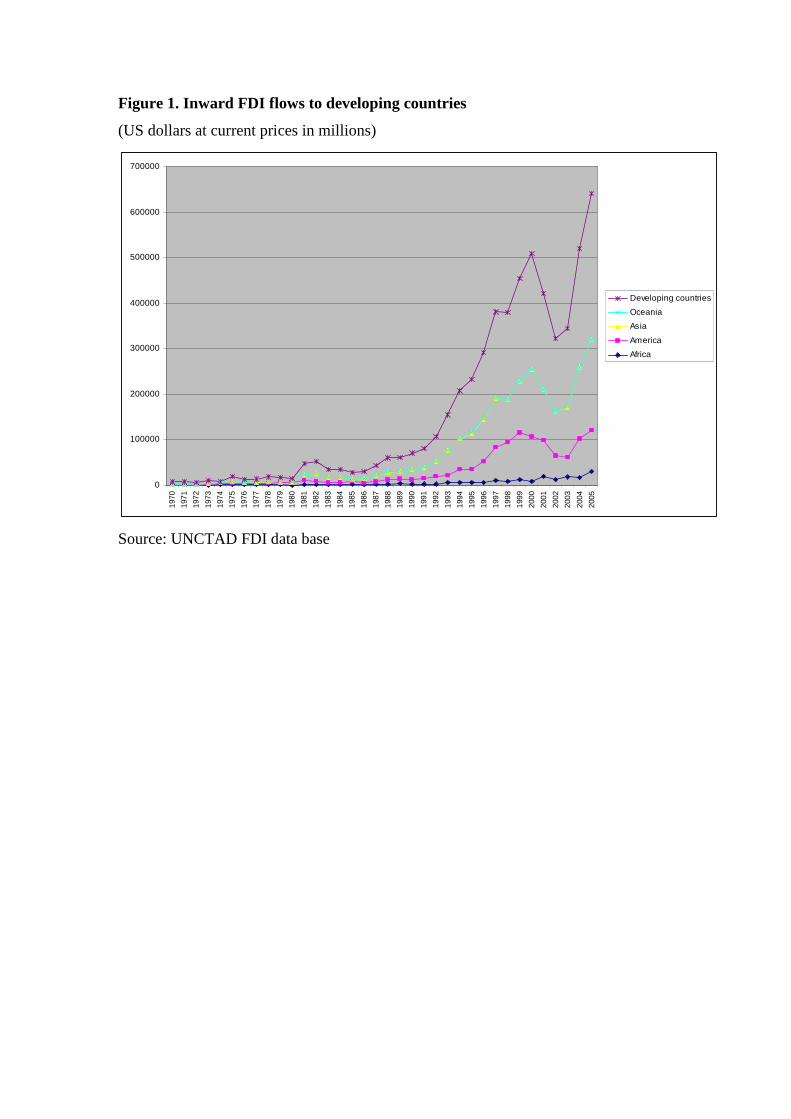
Figure 1. Inward FDI flows to developing countries

(US dollars at current prices in millions)

0

100000

200000

300000

400000

500000

600000

70000019

70

1971

1972

1973

1974

1975

1976

1977

1978

1979

1980

1981

1982

1983

1984

1985

1986

1987

1988

1989

1990

1991

1992

1993

1994

1995

1996

1997

1998

1999

2000

2001

2002

2003

2004

2005

Developing countries

Oceania

Asia

America

Africa

Source: UNCTAD FDI data base

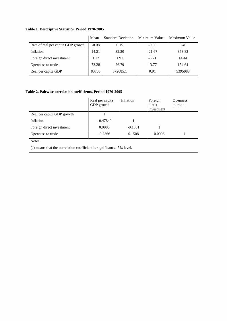
Table 1. Descriptive Statistics. Period 1970-2005

Mean Standard Deviation Minimum Value Maximum Value

Rate of real per capita GDP growth -0.08 0.15 -0.80 0.40

Inflation 14.21 32.20 -21.67 373.82

Foreign direct investment 1.17 1.91 -3.71 14.44

Openness to trade 73.28 26.79 13.77 154.64

Real per capita GDP 83705 572685.1 0.91 5395983

Table 2. Pairwise correlation coefficients. Period 1970-2005

Real per capita GDP growth

Inflation Foreign direct investment

Openness to trade

Real per capita GDP growth 1

Inflation -0.4784a 1

Foreign direct investment 0.0986 -0.1881 1

Openness to trade -0.2366 0.1508 0.0996 1

Notes

(a) means that the correlation coefficient is significant at 5% level.

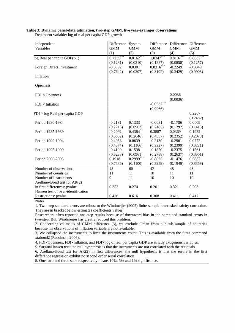
Table 3: Dynamic panel-data estimation, two-step GMM, five year-averages observations Dependent variable: log of real per capita GDP growth Independent Variables

Difference GMM (1)

System GMM (2)

Difference GMM (3)

Difference GMM (4)

Difference GMM (5)

0.7235*** 0.8162*** 1.0347*** 0.8107*** 0.8652*** log Real per capita GDP(t-1) (0.1281) (0.0210) (0.1387) (0.0858) (0.1257) -0.3992 0.0301 0.8316*** -0.2249 -0.8349 Foreign Direct Investment (0.7642) (0.0307) (0.3192) (0.3429) (0.9903) Inflation Openness 0.0036 FDI × Openness (0.0036) -0.0537*** FDI × Inflation (0.0066) 0.2267 FDI × log Real per capita GDP (0.2482) -0.2181 0.1333 -0.0081 -0.1786 0.0009 Period 1980-1984 (0.2215) (0.0962) (0.2185) (0.1292) (0.1415) -0.2092 0.4384* 0.3887 0.0369 0.1932 Period 1985-1989 (0.5662) (0.2646) (0.4557) (0.2352) (0.2078) -0.4956 0.0639 -0.2139 -0.2901 0.0772 Period 1990-1994 (0.4374) (0.1166) (0.2227) (0.2399) (0.3221) -0.4100 0.1538 -0.1850 -0.2375 0.1561 Period 1995-1999 (0.3238) (0.0961) (0.2788) (0.2637) (0.3501) 0.1918 0.2999*** -0.8025 -0.1476 0.5862 Period 2000-2005 (0.7586) (0.1100) (0.3959) (0.1949) (0.8369)

Number of observations 48 60 42 48 48 Number of countries 11 11 10 11 11 Number of instruments 9 11 10 10 10 Arellano-Bond test for AR(2) in first differences: pvalue

0.353

0.274

0.201

0.321

0.293

Hansen test of over-identification Restrictions: pvalue

0.426

0.616

0.308

0.411

0.417

Notes 1. Two-step standard errors are robust to the Windmeijer (2005) finite-sample heteroskedasticity correction. They are in bracket below estimates coefficients values. Researchers often reported one-step results because of downward bias in the computed standard errors in two-step. But, Windmeijer has greatly reduced this problem. 2. Concerning estimates of GMM difference (3), we exclude Oman from our sub-sample of countries because his observations of inflation variable are not available. 3. We collapsed the instruments to limit the instruments count. This is available from the Stata command xtabond2 (Roodman, 2006). 4. FDI×Openness, FDI×Inflation, and FDI× log of real per capita GDP are strictly exogenous variables. 5. Sargan/Hansen test: the null hypothesis is that the instruments are not correlated with the residuals. 6. Arellano-Bond test for AR(2) in first differences: the null hypothesis is that the errors in the first difference regression exhibit no second order serial correlation. 8. One, two and three stars respectively means 10%, 5% and 1% significance.

Table A.1: Dynamic panel-data estimation, two-step GMM, five year-averages observations Dependent variable: log of real per capita GDP growth

Independent Variables

Difference GMM (1)

System GMM (2)

Difference GMM (3)

Difference GMM (4)

Difference GMM (5)

0.7994*** 0.8385*** 1.0709*** 0.8061*** 1.0425*** log Initial real per capita GDP (0.1318) (0.0273) (0.1414) (0.0968) (0.2044) -0.1136 0.0206 1.0246** -0.4567 -3.0588 Foreign Direct Investment (0.2927) (0.0358) (0.4046) (0.4551) (2.5618) 0.0058 FDI × Openness (0.0050) -0.0671*** FDI × Inflation (0.0138) 0.8017 FDI × log Real per capita GDP (0.6657) -0.1958 0.1528 0.1404 -0.1647 0.5511 Period 1980-1984 (0.1447) (0.1245) (0.2910) (0.1791) (0.6502) -0.2439 0.2814 0.5751 -0.1249 0.6304 Period 1985-1989 (0.2934) (0.2460) (0.4562) (0.2355) (0.8188) -0.5894 -0.0178 -0.1836 -0.4490 0.9853 Period 1990-1994 (0.4285) (0.1983) (0.3747) (0.3543) (1.1746) -0.5898 0.0051 -0.2391 -0.5224 1.1356 Period 1995-1999 (0.4792) (0.1347) (0.4675) (0.4324) (1.4157) -0.1661 0.2321* -0.9419** -0.2866 2.7015 Period 2000-2005 (0.2276) (0.1381) (0.4817) (0.3549) (2.4176)

Number of observations 48 60 42 48 48 Number of countries 11 11 10 11 11 Number of instruments 9 11 10 10 10 Arellano-Bond test for AR(2) in first differences: pvalue

0.379

0.449

0.652

0.397

0.366

Hansen test of over-identification Restrictions: pvalue

0.344

0.361

0.501

0.311

0.338

Notes 1. Two-step standard errors are robust to the Windmeijer (2005) finite-sample heteroskedasticity correction. They are in bracket below estimates coefficients values. Researchers often reported one-step results because of downward bias in the computed standard errors in two-step. But, Windmeijer has greatly reduced this problem. 2. Concerning estimates of GMM difference (3), we exclude Oman from our sub-sample of countries because his observations of inflation variable are not available. 3. We collapsed the instruments to limit the instrument count. This is available from the Stata command xtabond2 (Roodman, 2006). 4. FDI×Openness, FDI×Inflation, and FDI× log of real per capita GDP are strictly exogenous variables. 5. Sargan/Hansen test: the null hypothesis is that the instruments are not correlated with the residuals. 6. Arellano-Bond test for AR(2) in first differences: the null hypothesis is that the errors in the first difference regression exhibit no second order serial correlation. 8. One, two and three stars respectively means 10%, 5% and 1% significance.

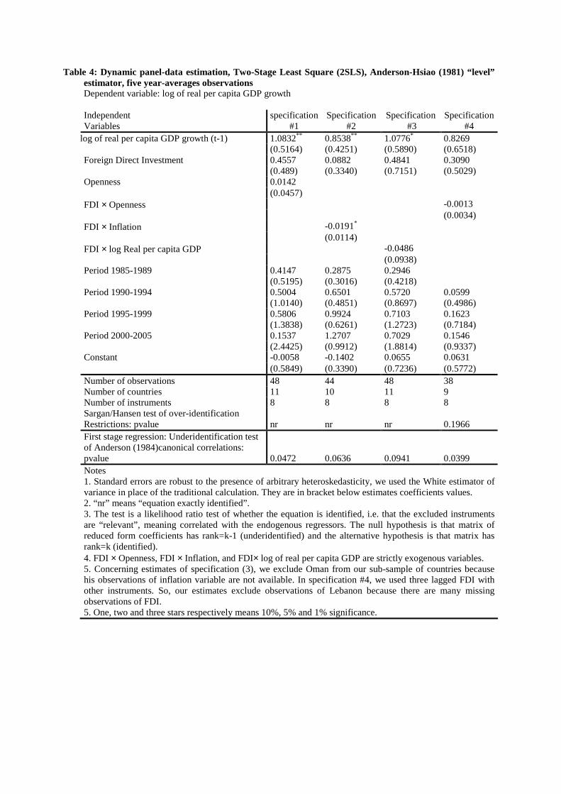
Table 4: Dynamic panel-data estimation, Two-Stage Least Square (2SLS), Anderson-Hsiao (1981) “level” estimator, five year-averages observations Dependent variable: log of real per capita GDP growth Independent Variables

specification #1

Specification #2

Specification #3

Specification #4

1.0832** 0.8538** 1.0776* 0.8269 log of real per capita GDP growth (t-1) (0.5164) (0.4251) (0.5890) (0.6518) 0.4557 0.0882 0.4841 0.3090 Foreign Direct Investment (0.489) (0.3340) (0.7151) (0.5029) 0.0142 Openness (0.0457) -0.0013 FDI × Openness (0.0034) -0.0191* FDI × Inflation (0.0114) -0.0486 FDI × log Real per capita GDP (0.0938) 0.4147 0.2875 0.2946 Period 1985-1989 (0.5195) (0.3016) (0.4218) 0.5004 0.6501 0.5720 0.0599 Period 1990-1994 (1.0140) (0.4851) (0.8697) (0.4986) 0.5806 0.9924 0.7103 0.1623 Period 1995-1999 (1.3838) (0.6261) (1.2723) (0.7184) 0.1537 1.2707 0.7029 0.1546 Period 2000-2005 (2.4425) (0.9912) (1.8814) (0.9337) -0.0058 -0.1402 0.0655 0.0631 Constant (0.5849) (0.3390) (0.7236) (0.5772)

Number of observations 48 44 48 38 Number of countries 11 10 11 9 Number of instruments 8 8 8 8 Sargan/Hansen test of over-identification Restrictions: pvalue

nr

nr

nr

0.1966

First stage regression: Underidentification test of Anderson (1984)canonical correlations: pvalue

0.0472

0.0636

0.0941

0.0399

Notes 1. Standard errors are robust to the presence of arbitrary heteroskedasticity, we used the White estimator of variance in place of the traditional calculation. They are in bracket below estimates coefficients values. 2. “nr” means “equation exactly identified”. 3. The test is a likelihood ratio test of whether the equation is identified, i.e. that the excluded instruments are “relevant”, meaning correlated with the endogenous regressors. The null hypothesis is that matrix of reduced form coefficients has rank=k-1 (underidentified) and the alternative hypothesis is that matrix has rank=k (identified). 4. FDI × Openness, FDI × Inflation, and FDI× log of real per capita GDP are strictly exogenous variables. 5. Concerning estimates of specification (3), we exclude Oman from our sub-sample of countries because his observations of inflation variable are not available. In specification #4, we used three lagged FDI with other instruments. So, our estimates exclude observations of Lebanon because there are many missing observations of FDI. 5. One, two and three stars respectively means 10%, 5% and 1% significance.