Fractional translational diffusion of a Brownian particle in a double well potential

Yuri P. KalmykovLaboratoire Mathématiques et Physique des Systèmes, Université de Perpignan, 52, Avenue de Paul Alduy,

66860 Perpignan Cedex, France

William T. CoffeyDepartment of Electronic and Electrical Engineering, Trinity College, Dublin 2, Ireland

Serguey V. TitovInstitute of Radio Engineering and Electronics of the Russian Academy of Sciences, Vvedenskii Square 1, Fryazino, Moscow Region,

141190, Russian Federation�Received 24 March 2006; published 11 July 2006�

The fractional translational diffusion of a particle in a double-well potential �excluding inertial effects� isconsidered. The position correlation function and its spectrum are evaluated using a fractional probabilitydensity diffusion equation �based on the diffusion limit of a fractal time random walk�. Exact and approximatesolutions for the dynamic susceptibility describing the position response to a small external field are obtained.The exact solution is given by matrix continued fractions while the approximate solution relies on the expo-nential separation of the time scales of the fast “intrawell” and low overbarrier relaxation processes associatedwith the bistable potential. It is shown that knowledge of the characteristic relaxation times for normaldiffusion allows one to predict accurately the anomalous relaxation behavior of the system for all relevant timescales.

DOI: 10.1103/PhysRevE.74.011105 PACS number�s�: 05.40.�a, 05.45.Df

I. INTRODUCTION

Relaxation and diffusion processes in complex disorderedsystems such as amorphous polymers, glass forming liquids,etc., exhibit temporal nonlocal behavior arising from ener-getic disorder causing obstacles or traps both slowing downthe motion of the particle and introducing memory effects.The memory effects can be described by a fractional diffu-sion equation incorporating a waiting time probability den-sity function �1,2� governing the random time intervals be-tween single microscopic jumps of the particles. Thefractional diffusion equation stems from the integral equationfor a continuous time random walk �CTRW� �3,4�. The situ-ation is thus unlike that in a conventional random walkwhich is characterized by a microscopic time scale smallcompared to the observation time. The microscopic time inthe conventional random walk is the time the random walkertakes to make a single microscopic jump. In this context oneshould recall that the Einstein theory of the normal Brownianmotion relies on the diffusion limit of a discrete time randomwalk. Here the random walker makes a jump of a fixed meansquare length in a fixed time thus the only random variable isthe direction of the walker, leading automatically via the cen-tral limit theorem �in the limit of a large sequence of jumps�to the Wiener process describing the Brownian motion. TheCTRW, on the other hand, was introduced by Montroll andWeiss �4� as a way of rendering time continuous in a randomwalk without necessarily appealing to the diffusion limit. Inthe most general case of the CTRW, the random walker mayjump an arbitrary length in arbitrary time. However, the jumplength and jump time random variables are not statisticallyindependent �1,5,6�. In other words a given jump length ispenalized by a time cost, and vice versa. A simple case of theCTRW arises when one assumes that the jump length and

jump time random variables are decoupled. Thus the jumplength variances are always finite; however, the jump timesmay be arbitrarily long so that they obey a Lévy distributionwith its characteristic long tail �5,6�. Thus the jump lengthdistribution ultimately becomes Gaussian with finite jumplength variance, while the mean waiting time between jumpsdiverges due to the underlying Lévy waiting time distribu-tion. Such walks, which possess a discrete hierarchy of timescales, not all of which have the same probability of occur-rence, are known as fractal time random walks �5�. In thelimit of a large sequence of jump times, they yield a frac-tional Fokker-Planck equation in configuration space �5,7�.

Now the relevant fractional diffusion �Fokker-Planck�equation for the distribution function W�x , t� of the one-dimensional noninertial translational motion of a particle in apotential V�x , t� may be written as �1,2�

�W�x,t��t

= 0Dt1−�K�

�

�x� �

�xW�x,t� +

W�x,t�kT

�

�xV�x,t�� .

�1�

Here x specifies the position of the particle at time t,−��x��, kT is the thermal energy, and K�=�� /kT is ageneralized diffusion coefficient, and �� is a generalized vis-cous drag coefficient arising from the heat bath. The operator

0Dt1−�� �

�t 0Dt−� in Eq. �1� is given by the convolution �the

Riemann-Liouville fractional integral definition� �1�

0Dt−�W�x,t� =

1

�����0

t W�x,t��dt�

�t − t��1−� , �2�

where ��z� is the � function �8�. The physical meaning of theparameter � is the order of the fractional derivative in the

PHYSICAL REVIEW E 74, 011105 �2006�

1539-3755/2006/74�1�/011105�7� ©2006 The American Physical Society011105-1

ractional differential equation describing the continuum limitof a random walk with a chaotic set of waiting times �oftenknown as a fractal time random walk�. Values of � in therange 0���1 correspond to subdiffusion phenomena��=1 corresponds to normal diffusion�. However, a morephysically useful definition of � is as the fractal dimensionof the set of waiting times. The fractal dimension is the scal-ing of the waiting time segments in the random walk withmagnification of the walk. Thus, � measures the statisticalself-similarity �or how the whole resembles its individualconstituent parts �5�� of the waiting time segments. In orderto construct such an entity in practice a whole discrete hier-archy of time scales such as will arise from energetic disor-der is needed. For example a fractal time Poisson process �5�with a waiting time distribution assumes the typical form ofa Lévy stable distribution in the limit of large �. This isexplicitly discussed in Ref. �5� where a formula for � isgiven and is also discussed in Ref. �9�. The fractal time pro-cess is essentially generated by the energetic disorder treatedas far as the ensuing temporal behavior is concerned by con-sidering jumps over the wells of a chaotic potential barrierlandscape.

The fractional diffusion equation �1� can in principle besolved by the same methods as the normal Fokker-Planckequation. However, to the best of our knowledge no explicitsolutions for the fractional translational diffusion in a poten-tial have ever been presented. The only exception appears tobe a solution for the harmonic potential given by Metzler etal. �10� in terms of an eigenfunction expansion with Mittag-Leffler temporal behavior. This approach has recently beenextended to the analogous fractional rotational diffusionmodels in a periodic potential by Coffey et al. �11–13�.There, the authors have developed effective methods of so-lution of fractional diffusion equations based on ordinary andmatrix continued fractions �as is well known the continuedfractions are an extremely powerful tool in the solution ofnormal diffusion equations �7,14��. Here we further general-ize the methods of Coffey et al. �11–13� for fractional trans-lational diffusion problems. As a particular example, we shallpresent both exact and approximate solutions for the anoma-lous diffusion of a particle in a double-well potential, viz.

V�x� =1

2ax2 +

1

4bx4, �3�

where a and b are constants. The model of normal diffusionin the 2–4 potential Eq. �3� is almost invariably used to de-scribe the noise driven motion in bistable physical andchemical systems. Examples are such diverse subjects assimple isometrization processes �15–19�, chemical reactionrate theory �20–28�, bistable nonlinear oscillators �29–31�,second order phase transitions �32�, nuclear fission and fu-sion �33,34�, stochastic resonance �35,36�, etc.

The normal diffusion in the 2–4 potential in the very highdamping limit, where the inertia of the particle may be ne-glected, has been extensively studied either by using theKramers escape rate theory or by solution of the appropriateFokker-Planck �Smoluchowski� equation �see, e.g., Refs.�7,22,25,36–38�, and references cited therein�. In the VHDlimit, the conventional analysis of the problem proceeds

from the Smoluchowski equation by either rendering thatequation as a Sturm-Liouville problem �e.g., Refs. �25,39��or by the solution of an infinite hierarchy of lineardifferential-recurrence relations for statistical moments �e.g.,Refs. �40,41��. The same methods may be used if the inertialeffects are included �see e.g., Refs. �42,43��. The fractionaldiffusion equation �1� can in principle be treated in a likemanner. The subdiffusion in the double-well potential Eq. �3�has been considered in Refs. �44,45� in terms of an eigen-function expansion with Mittag-Leffler temporal behavior. InRefs. �44,45�, the authors mainly studied the effect of bound-ary conditions on the transition probability density. In con-trast, the purpose of the present paper is to ascertain how theanomalous diffusion in a bistable potential, b0 and a�0,modifies the behavior of the position correlation functionC��t�= x�0�x�t�0 / x2�0�0 and its spectra �which character-ize the anomalous relaxation�. We shall give exact and ap-proximate solutions for these quantities. Furthermore, weshall demonstrate that the characteristic times of the normaldiffusion process, namely, the inverse of the smallest nonva-nishing eigenvalue of the Fokker-Planck operator, the inte-gral and effective relaxation times, obtained in Ref. �7�, alsoallow us to describe the anomalous relaxation behavior.

II. BASIC EQUATIONS

By using dimensionless variables and parameters asdefined in �7,38�, viz.

V�y� =V�x�kT

= Ay2 + By4, y =x

x201/2 , A =

ax20

2kT,

B =bx20

2

4kT,

the fractional Fokker-Planck equation becomes

�W�y,t��t

= �−�0Dt

1−� �

�y� �

�yW�y,t� + W�y,t�

�

�yV�y,t�� ,

�4�

where �= x20 /K1 has the meaning of the characteristic in-tertrapping time �waiting time between jumps�, K1 is the dif-fusion coefficient for normal diffusion, and the angularbrackets �·�0=Z−1�−�

� �·�e−V�y�dy mean equilibrium en-semble averages. Here Z is the partition function given by forA�0 �which is the case of greatest interest� �7�

Z = �−�

�

e−V�y�dy = ��2B�−1/4eQ/2D−1/2�− �2Q� , �5�

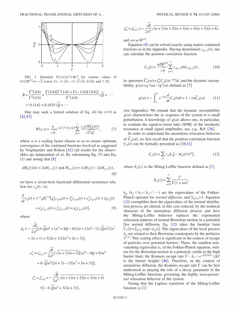
where Dv�z� are Whitaker’s parabolic cylinder functions oforder v �8� and Q=A2 /4B is the barrier height for the poten-tial V�y�=Ay2+By4 �see Fig. 1�. The normalization conditiony20=1 implies that the constants A and B are now not in-dependent �7�

B = B�Q� =1

8

D−3/22 �sgn�A��2Q�

D−1/22 �sgn�A��2Q�

. �6�

For A�0 and large barriers �Q�1�, B Q while for small Q

KALMYKOV, COFFEY, AND TITOV PHYSICAL REVIEW E 74, 011105 �2006�

011105-2

B =�2�3/4��2�1/4�

+��3/4���2�1/4� + ��− 1/4���3/4��

�3�1/4��Q + ¯

� 0.1142 + 0.1835�Q + ¯

One may seek a formal solution of Eq. �4� for t�0 as�42,43�

W�y,t� =

�e−� 2y2+V�y��/2�

q=1

�cq�t�Hq� y�

�2qq!, �7�

where is a scaling factor chosen so as to ensure optimumconvergence of the continued fractions involved as suggestedby Voigtlaender and Risken �42� �all results for the observ-ables are independent of �. By substituting Eq. �7� into Eq.�1� and noting that �8�

dHn�z�/dz = 2nHn−1�z� and Hn+1�z� = 2zHn�z� − 2nHn−1�z� ,

�8�

we have a seven-term fractional differential recurrence rela-tion for cq�t�, viz.

d

dtcq�t� = �−�

0Dt1−��gq

+cq+6�t� + fq+cq+4�t� + eq

+cq+2�t� + dqcq�t�

+ eq−cq−2�t� + fq

−cq−4�t� + gq−cq−6�t�� , �9�

where

dn = −�B

2�6 �4�Q�6 + ��4 + 4Q − 6��2n + 1��4− 12�Q�2�2n2

+ 2n + 1� + 5�2n + 1��2n2 + 2n + 3�� ,

en+ = en+2

− =�B

2�6 ���n + 1��n + 2����4 − 4Q + 6��4

+ 8�Q�2�2n + 3� − 15�n2 + 3n + 3��� ,

fn+ = fn+2

− = −�B

2�6��n + 1��n + 2��n + 3��n + 4�

��− 4�Q�2 + 3�2n + 5�� ,

gn+ = gn+2

− = −�B

2�6��n + 1��n + 2��n + 3��n + 4��n + 5��n + 6� ,

and �= /B1/4.Equation �9� can be solved exactly using matrix continued

fractions as in the Appendix. Having determined c2q−1�t�, onecan calculate the position correlation function

C��t� =�ZB1/4

��q=1

�

c2q−1�0�c2q−1�t� , �10�

its spectrum C����=�0�C��t�e−i�tdt, and the dynamic suscep-

tibility ����=�����− i����� defined as �7�

���� = − �0

�

e−i�t d

dtC��t�dt = 1 − i�C���� �11�

�see Appendix�. We remark that the dynamic susceptibility���� characterizes the ac response of the system to a smallperturbation. A knowledge of ���� allows one, in particular,to evaluate the signal-to-noise ratio �SNR� of the stochasticresonance at small signal amplitudes, see, e.g., Ref. �36�.

In order to understand the anomalous relaxation behavior

of C����, we first recall that the position correlation functionC��t� can be formally presented as �10,11�

C��t� = �p

cpE��− ��p�t/���� , �12�

where E��z� is the Mittag-Leffler function defined as �1�

E��z� = �n=0

�zn

��1 + n��,

�p ��1��2��3� ¯ � are the eigenvalues of the Fokker-Planck operator for normal diffusion, and �pcp=1. Equation�12� exemplifies how the eigenvalues of the normal distribu-tion process are altered, in this case reduced, by the nonlocalcharacter of the anomalous diffusion process and howthe Mittag-Leffler behavior replaces the exponentialrelaxation patterns of normal Brownian motion in a potential�for normal diffusion, Eq. �12� takes the familiar formC1�t�=�pcp exp�−�pt��. The eigenvalues of the local process�p are related to their Brownian counterparts by the prefactor�1−�. This scaling effect is significant in the context of escapeof particles over potential barriers. There, the smallest non-vanishing eigenvalue �1 of the Fokker-Planck equation, writ-ten for the Brownian motion in a potential, yields in the highbarrier limit, the Kramers escape rate � �1 e−�V/�kT� ��Vis the barrier height� �46�. Therefore, in the context ofanomalous diffusion, the Kramers escape rate � can be bestunderstood as playing the role of a decay parameter in theMittag-Leffler functions governing the highly nonexponen-tial relaxation behavior of the system.

Noting that the Laplace transform of the Mittag-Lefflerfunction is �1�

FIG. 1. Potential V�y�=Ay2+By4 for various values ofA / �2B1/2�=−�2 �curve 1�, −1 �2�, −1/�2 �3�, 0 �4�, and 1 �5�.

FRACTIONAL TRANSLATIONAL DIFFUSION OF A¼ PHYSICAL REVIEW E 74, 011105 �2006�

011105-3

�0

�

e−stE��− �p��t/����dt =1

s + �p��s�1−� ,

Eqs. �11� and �12� and yield

���� = �p

cp

1 + �i����/���p�. �13�

In the low- �→0� and high- ��→�� frequency limits, thebehavior of the susceptibility may now be readily evaluated.We have from Eq. �11� for �→0 and for �→�, respectively

���� � 1 −�int

��i���� + ¯ , �14�

���� �

�i�����ef+ ¯ , �15�

where the parameters �int and �ef are given by

�int = �p

cp/�p and �ef = 1/�p

cp�p. �16�

For normal diffusion, these parameters correspond to the cor-relation �or integral relaxation� time �int=�0

�C1�t�dt �the areaunder the correlation function C1�t�=�pcpe−�pt� and the ef-

fective relaxation time �ef =−1/ C1�0� �which gives preciseinformation on the initial decay of C1�t��. We remark thatno such characteristic times exist in anomalous diffusion���1�. This is obvious from the long time inverse powerlaw behavior of the Mittag-Leffler function. In anomalousdiffusion, the times �1

−1, �int, and �ef are always parameters ofthe normal diffusion. They exist because in normal diffusionan underlying microscopic time scale exists, namely the du-ration of an elementary jump, characteristic of the discretetime random walk as used by Einstein.

III. TWO MODE APPROXIMATION FOR C�„t…

As we shall see, two bands appear in the spectrumof �����. The low-frequency band is due to the slowest�overbarrier� relaxation mode; the characteristic frequency�c and the half width of this band are determined by thesmallest nonvanishing eigenvalue �1. Thus, the anomalouslow frequency behavior is dominated by the barrier crossingmode as in the normal diffusion. The high-frequency band isdue to “intrawell” modes corresponding to the eigenvalues�k �k�1�. These near degenerate intrawell modes are indis-tinguishable in the frequency spectrum of ����� appearingmerely as a single high-frequency band. As shown byKalmykov et al. �11�, the susceptibility ���� can be effec-tively described via a two mode approximation, viz.

���� =�1

1 + �i�/�c�� +1 − �1

1 + �i�/�W�� , �17�

where the characteristic frequencies �c and �W are given by

�c = �−1���1�1/�, �W = �−1��/�W�1/�. �18�

The parameters �1 and �W are defined in terms of the char-acteristic times of the normal diffusion �the integral relax-

ation time �int, the effective relaxation time �ef, and the in-verse of the smallest nonvanishing eigenvalue 1/�1� �7,11�

�1 =�int/�ef − 1

�1�int − 2 + 1/��1�ef�, �W =

�1�int − 1

�1 − 1/�ef. �19�

In the time domain, such a bimodal approximation is equiva-lent to assuming that the correlation function C��t� yieldedby the exact Eq. �12� �which in general comprises an infinitenumber of Mittag-Leffler functions� may be approximated bytwo Mittag-Leffler functions only, viz.

C��t� � �1E��− �t/�����1� + �1 − �1�E��− �t/����/�W� .

�20�

The characteristic times 1/�1, �int, and �ef for the normalBrownian motion in a double-well potential Eq. �3� havebeen obtained in Refs. �38,41� �see also �7�, Chapter 6�. Herewe simply use known equations for �1, �int, and �ef for nor-mal diffusion in order to predict the anomalous relaxationbehavior. The �int and �ef for normal diffusion may be ex-pressed in exact closed form, viz. ��7�, Chapter 6�

�ef = � , �21�

�int = ��eQ/2D−1/2�− �2Q�

23/4D−3/22 �− �2Q�

�0

�

e�s − �Q�2�1 − erf�s − �Q��2 ds

�s,

�22�

where erf�z�= 2�

�0ze−z2

dz is the error function �8�. The small-est nonvanishing eigenvalue �1 can be estimated in terms ofmatrix continued fractions from Eq. �34� of the Appendix.Moreover, for all values of Q, �1 can be evaluated with veryhigh accuracy from the approximate equation �7�

�1 =D−3/2�− �2Q�

�D−1/2�− �2Q�� eQ

1 + erf��Q��

0

� �0

�

e−�s − �Q�2−�t − �Q�2

�erf��2st�

�stdsdt�−1

. �23�

In the low temperature limit, Q�1, �1−1 and �int have the

simple asymptotic behavior �7,25�

1/�1 �eQ

4�2Q�1 +

5

8Q+ ¯ �, �24�

�int �eQ

4�2Q�1 +

1

2Q+ ¯ � .

Equations �17�–�24� allow one readily to estimate the quali-tative behavior of the susceptibility ���� and its characteris-tic frequencies �c and �W. In particular, Eqs. �18�–�21� and�24� yield simple asymptotic equations for the amplitude �1and characteristic frequencies �c and �W in the low tempera-ture limit �Q�1�, viz.

�1 1 − 1/�8Q�, �c �4�2Q/�1/�e−Q/�/�,

and �W �8Q�1/�/� . �25�

Equations �17�, �18�, �20�, and �25� allows one to readily

KALMYKOV, COFFEY, AND TITOV PHYSICAL REVIEW E 74, 011105 �2006�

011105-4

evaluate ���� and C��t� at high barriers, Q�1.

IV. RESULTS AND DISCUSSION

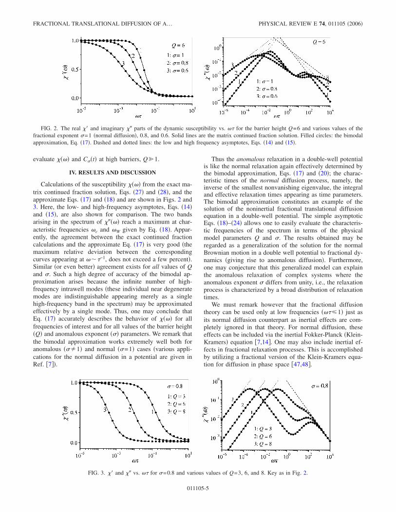
Calculations of the susceptibility ���� from the exact ma-trix continued fraction solution, Eqs. �27� and �28�, and theapproximate Eqs. �17� and �18� and are shown in Figs. 2 and3. Here, the low- and high-frequency asymptotes, Eqs. �14�and �15�, are also shown for comparison. The two bandsarising in the spectrum of ����� reach a maximum at char-acteristic frequencies �c and �W given by Eq. �18�. Appar-ently, the agreement between the exact continued fractioncalculations and the approximate Eq. �17� is very good �themaximum relative deviation between the correspondingcurves appearing at � �−1, does not exceed a few percent�.Similar �or even better� agreement exists for all values of Qand �. Such a high degree of accuracy of the bimodal ap-proximation arises because the infinite number of high-frequency intrawell modes �these individual near degeneratemodes are indistinguishable appearing merely as a singlehigh-frequency band in the spectrum� may be approximatedeffectively by a single mode. Thus, one may conclude thatEq. �17� accurately describes the behavior of ���� for allfrequencies of interest and for all values of the barrier height�Q� and anomalous exponent ��� parameters. We remark thatthe bimodal approximation works extremely well both foranomalous ���1� and normal ��=1� cases �various appli-cations for the normal diffusion in a potential are given inRef. �7��.

Thus the anomalous relaxation in a double-well potentialis like the normal relaxation again effectively determined bythe bimodal approximation, Eqs. �17� and �20�; the charac-teristic times of the normal diffusion process, namely, theinverse of the smallest nonvanishing eigenvalue, the integraland effective relaxation times appearing as time parameters.The bimodal approximation constitutes an example of thesolution of the noninertial fractional translational diffusionequation in a double-well potential. The simple asymptoticEqs. �18�–�24� allows one to easily evaluate the characteris-tic frequencies of the spectrum in terms of the physicalmodel parameters Q and �. The results obtained may beregarded as a generalization of the solution for the normalBrownian motion in a double well potential to fractional dy-namics �giving rise to anomalous diffusion�. Furthermore,one may conjecture that this generalized model can explainthe anomalous relaxation of complex systems where theanomalous exponent � differs from unity, i.e., the relaxationprocess is characterized by a broad distribution of relaxationtimes.

We must remark however that the fractional diffusiontheory can be used only at low frequencies ����1� just asits normal diffusion counterpart as inertial effects are com-pletely ignored in that theory. For normal diffusion, theseeffects can be included via the inertial Fokker-Planck �Klein-Kramers� equation �7,14�. One may also include inertial ef-fects in fractional relaxation processes. This is accomplishedby utilizing a fractional version of the Klein-Kramers equa-tion for diffusion in phase space �47,48�.

FIG. 2. The real �� and imaginary �� parts of the dynamic susceptibility vs. �� for the barrier height Q=6 and various values of thefractional exponent �=1 �normal diffusion�, 0.8, and 0.6. Solid lines are the matrix continued fraction solution. Filled circles: the bimodalapproximation, Eq. �17�. Dashed and dotted lines: the low and high frequency asymptotes, Eqs. �14� and �15�.

FIG. 3. �� and �� vs. �� for �=0.8 and various values of Q=3, 6, and 8. Key as in Fig. 2.

FRACTIONAL TRANSLATIONAL DIFFUSION OF A¼ PHYSICAL REVIEW E 74, 011105 �2006�

011105-5

Finally in view of previous work �49,50� in the theory ofanomalous translational diffusion we briefly allude to addi-tional mechanisms yielding anomalous diffusion in a poten-tial. Examples are time rescaled Brownian motion or gener-alized Langevin equations with nonwhite Gaussian noise�49,50� so that the memory function is no longer a � func-tion. Moreover the concept of a generalized Langevin equa-tion with friction term given by the Riemann-Liouville defi-nition of the fractional derivative has been used by Lutz �51�to analyze translational anomalous diffusion.

ACKNOWLEDGMENTS

The TCD Trust is gratefully acknowledged for financialsupport for S.V.T.

APPENDIX: MATRIX CONTINUED FRACTIONSOLUTION

Equation �9� can be rearranged as the set of matrix three-term recurrence equations

�d

dtCn�t� = �1−�

0Dt1−��Qn

−Cn−1�t� + QnCn�t�

+ Qn+Cn+1�t��, �n � 1� , �26�

where the column vectors Cn�t� and the matrices Qn, Qn+, Qn

−

are

Cn�t� = �c6n−5�t�c6n−3�t�c6n−1�t�

� ,

Qn = �d6n−5+ e6n−5

+ f6n−5+

e6n−5+ d6n−3

+ e6n−3+

f6n−5+ e6n−3

+ d6n−1+ � ,

Qn+ = �g6n−5

+ 0 0

f6n−3+ g6n−3

+ 0

e6n−1+ f6n−1

+ g6n−1+ � ,

Qn− = �Qn−1

+ �T

�the sign “T” designates transposition�. Now by one-sidedFourier transformation, Eq. �26� can be rearranged as the setof matrix three-term recurrence equations

�i����Cn��� − ��i����−1Cn�0� = QnCn��� + Qn+Cn+1���

+ Qn−Cn−1��� , �27�

where Cn���=�0�Cn�t�e−i�tdt. By invoking the general

method �7,14� for solving the tridiagonal matrix recurrence

Eq. �26� and noting that C0���=0, we have the exact solu-

tion for C1��� in terms of matrix continued fractions, viz.

C1��� = ��i����−1�1�i���C1�0�

+ �n=2

� ��k=2

n

Qk−1+ �k�i���Cn�0�� , �28�

where �n��� are the matrix continued fractions defined bythe recurrence equation

�n��� = ��i����I − Qn − Qn+�n+1���Qn+1

− �−1. �29�

All other Cn��� can be calculated from the recurrence Eq.�27�. The spectrum of the equilibrium correlation positionfunction C��t� is then given by

C���� =�ZB1/4

��n=1

�

CnT�0�Cn���

=�ZB1/4

��q=1

�

c2q−1�0�c2q−1��� , �30�

where the sign T �transpose� designates transformation of acolumn vector Cn�0� to a row vector. Equation �30� followsfrom the definition of the correlation function C��t� �42�, viz.

C��t� = y�0�y�t�0 = �−�

� �−�

�

yy0W�y,t�y0,0�W0�y0�dydy0,

�31�

where y0=y�0�, W0�y0�=e−Ay02−By0

4/Z is equilibrium �Boltz-

mann� distribution function, and W�y , t �y0 ,0� is the transi-tion probability, which satisfies Eq. �1� with the initial con-dition W�y ,0 �y0 ,0�=��y−y0� and is defined as

W�y,t�y0,0� =

�e− 2�y2+y0

2�/2−�V�y�−V�y0��/2

��q,p=1

��G�t��q,pHq� y�Hp� y0�

�2q+pq!p!.

Here

�G�t��q,p =

�2q+pq!p!�

−�

� �−�

�

Hq� y�Hp� y0�

�e− 2�y2+y02�/2+�V�y�−V�y0��/2W�y,t�y0,0�dydy0

are the matrix elements of the system matrix G�t�. The co-efficients cq�t� are given in terms of elements of the systemmatrix G as

cq�t� = �p=1

�

�G�t��q,pcp�0� �32�

with the initial conditions

cp�0� =1

Z�2pp!B�

−�

�

xHp��x�e−��2x2−2�Qx2+x4�/2dx . �33�

KALMYKOV, COFFEY, AND TITOV PHYSICAL REVIEW E 74, 011105 �2006�

011105-6

Noting Eq. �30�, the correlation time �int= C1�0� and the

effective relaxation time �ef =−1/ C1�0� for normal diffusion,�=1, can be calculated in terms of matrix continued frac-tions as

�int =�ZB1/4

��n=1

�

CnT�0�Cn�0� ,

�ef = − ��ZB1/4

��n=1

�

CnT�0�Cn�0��−1

;

the smallest nonvanishing eigenvalue �1 can be evaluatedfrom the secular equation �7,14�

det��1�I + Q1 + Q1+�2�− �1�Q2

−� = 0. �34�

�1� R. Metzler and J. Klafter, Phys. Rep. 339, 1 �2000�.�2� R. Metzler and J. Klafter, Adv. Chem. Phys. 116, 223 �2001�.�3� E. W. Montroll and M. F. Shlesinger, On the Wonderful World

of Random Walks, edited by J. L. Lebowitz and E. W. Mon-troll, in Non Equilibrium Phenomena II from Stochastics toHydrodynamics �Elsevier Science Publishers, BV, Amsterdam,1984�.

�4� E. W. Montroll and G. H. Weiss, J. Math. Phys. 6, 167 �1965�.�5� W. Paul and J. Baschnagel, Stochastic Processes from Physics

to Finance �Springer Verlag, Berlin, 1999�.�6� B. J. West, M. Bologna, and P. Grigolini, Physics of Fractal

Operators �Springer, New York, 2003�.�7� W. T. Coffey, Yu. P. Kalmykov, and J. T. Waldron, The Lange-

vin Equation, 2nd edition �World Scientific, Singapore, 2004�.�8� Handbook of Mathematical Functions, edited by M.

Abramowitz and I. Stegun �Dover, New York, 1964�.�9� V. V. Novikov and V. P. Privalko, Phys. Rev. E 64, 031504

�2001�; V. V. Novikov, K. W. Wojciechowski, and V. P.Privalko, J. Phys.: Condens. Matter 12, 4869 �2000�.

�10� R. Metzler, E. Barkai, and J. Klafter, Phys. Rev. Lett. 82, 3563�1999�.

�11� Yu.P. Kalmykov, W. T. Coffey, and S. V. Titov, Phys. Rev. E69, 021105 �2004�.

�12� W. T. Coffey, Yu. P. Kalmykov, S. V. Titov, and J. K. Vij,Phys. Rev. E 72, 011103 �2005�.

�13� W. T. Coffey, Yu. P. Kalmykov, and S. V. Titov, Adv. Chem.Phys. 133, 285 �2006�.

�14� H. Risken, The Fokker-Planck Equation, 2nd edition�Springer, Berlin, 1989�.

�15� D. Chandler, J. Chem. Phys. 68, 2959 �1978�.�16� B. J. Berne, J. L. Skinner, and P. G. Wolynes, J. Chem. Phys.

73, 4314 �1980�.�17� D. L. Hasha, T. Eguchi, and J. Jonas, J. Am. Chem. Soc. 73,

1571 �1981�; ibid. 104, 2290 �1982�.�18� D. K. Garrity and J. L. Skinner, Chem. Phys. Lett. 95, 46

�1983�.�19� B. Carmeli and A. Nitzan, J. Chem. Phys. 80, 3596 �1984�.�20� H. A. Kramers, Physica �Amsterdam� 7, 284 �1940�.�21� H.C. Brinkman, Physica �Amsterdam� 22, 29 �1956�; ibid. 22,

149 �1956�.�22� C. Blomberg, Physica A 86, 49 �1977�; ibid. 86, 67 �1977�.�23� P. B. Visscher, Phys. Rev. B 14, 347 �1976�.�24� J. L. Skinner and P. G. Wolynes, Chem. Phys. 69, 2143

�1978�; J. Chem. Phys. 72, 4913 �1980�.

�25� R. S. Larson and M. D. Kostin, J. Chem. Phys. 69, 4821�1978�; , ibid. 72, 1392 �1980�.

�26� S. C. Northrup and J. T. Hynes, Chem. Phys. 69, 5246 �1978�;J. Chem. Phys. 69, 5261 �1978�; ibid. 73, 2700 �1980�; R. F.Grote and J. T. Hynes, ibid. 73, 2715 �1980�.

�27� M. Mangel, J. Chem. Phys. 72, 6606 �1980�.�28� K. Schulten, Z. Schulten, and A. Szabo, J. Chem. Phys. 74,

4426 �1981�.�29� M. Bixon and R. Zwanzig, J. Stat. Phys. 3, 245 �1971�.�30� M. I. Dykman, S. M. Soskin, and M. A. Krivoglaz, Physica A

133, 53 �1985�.�31� P. Hänggi, Phys. Lett. 78A, 304 �1980�.�32� J. A. Krumhansl and J. R. Schriefier, Phys. Rev. B 11, 3535

�1975�.�33� J. D. Bao and Y. Z. Zhuo, Phys. Rev. C 67, 064606 �2003�.�34� V. M. Kolomietz, S. V. Radionov, and S. Shlomo, Phys. Rev. C

64, 054302 �2001�.�35� M. I. Dykman, G. P. Golubev, D. G. Luchinsky, P. V. E. Mc-

Clintock, N. D. Stein, and N. G. Stocks, Phys. Rev. E 49, 1935�1994�.

�36� L. Gammaitoni, P. Hänggi, P. Jung, and F. Marchesoni, Rev.Mod. Phys. 70, 223 �1998�.

�37� W. T. Coffey, M. W. Evans, and P. Grigolini, MolecularDiffusion and Spectra �Wiley, New York, 1984�.

�38� A. Perico, R. Pratolongo, K. F. Freed, R. W. Pastor, and A.Szabo, J. Chem. Phys. 98, 564 �1993�.

�39� A. Schenzle and H. Brand, Phys. Rev. A 20, 1628 �1979�.�40� I. I. Fedchenia, J. Phys. A 25, 6733 �1992�.�41� Yu. P. Kalmykov, W. T. Coffey, and J. T. Waldron, J. Chem.

Phys. 105, 2112 �1996�.�42� K. Voigtlaender and H. Risken, J. Stat. Phys. 40, 397 �1985�;

Chem. Phys. Lett. 105, 506 �1984�.�43� Yu. P. Kalmykov, W. T. Coffey, and S. V. Titov, J. Chem. Phys.

124, 024107 �2006�.�44� F. So and K. L. Liu, Physica A 331, 378 �2004�.�45� C. W. Chow and K. L. Liu, Physica A 341, 8 �2004�.�46� P. Hänggi, P. Talkner, and M. Borcovec, Rev. Mod. Phys. 62,

251 �1990�.�47� E. Barkai and R. S. Silbey, J. Phys. Chem. B 104, 3866

�2000�.�48� R. Metzler and J. Klafter, J. Phys. Chem. B 104, 3851 �2000�.�49� K. G. Wang and C. W. Lung, Phys. Lett. A 151, 119 �1990�.�50� K. G. Wang, Phys. Rev. A 45, 833 �1992�.�51� E. Lutz, Phys. Rev. E 64, 051106 �2001�.

FRACTIONAL TRANSLATIONAL DIFFUSION OF A¼ PHYSICAL REVIEW E 74, 011105 �2006�

011105-7