Modelling the effects of a bushfire on erosion in a Mediterranean basin / Modélisation des impacts d'un incendie sur l'érosion dans un bassin Méditerranéen

This article was downloaded by: [North Dakota State University]On: 22 October 2014, At: 18:47Publisher: Taylor & FrancisInforma Ltd Registered in England and Wales Registered Number: 1072954 Registered office: MortimerHouse, 37-41 Mortimer Street, London W1T 3JH, UK

Hydrological Sciences JournalPublication details, including instructions for authors and subscription information:http://www.tandfonline.com/loi/thsj20

Modelling the effects of a bushfire on erosion in aMediterranean basin / Modélisation des impacts d'unincendie sur l'érosion dans un bassin MéditerranéenGian Vito Di Piazza , Costanza Di Stefano & Vito Ferroa Dipartimento di Ingegneria e Tecnologie Agro-Forestali, Facoltà di Agraria, Università diPalermo, Viale delle Scienze, I-90128 Palermo, Italy.b Dipartimento di Ingegneria e Tecnologie Agro-Forestali, Facoltà di Agraria, Universitàdi Palermo, Viale delle Scienze, I-90128 Palermo, Italy.c Dipartimento di Ingegneria e Tecnologie Agro-Forestali, Facoltà di Agraria, Università diPalermo, Viale delle Scienze, I-90128 Palermo, Italy.Published online: 15 Dec 2009.

To cite this article: Gian Vito Di Piazza , Costanza Di Stefano & Vito Ferro (2007) Modelling the effects of a bushfire onerosion in a Mediterranean basin / Modélisation des impacts d'un incendie sur l'érosion dans un bassin Méditerranéen ,Hydrological Sciences Journal, 52:6, 1253-1270, DOI: 10.1623/hysj.52.6.1253

To link to this article: http://dx.doi.org/10.1623/hysj.52.6.1253

PLEASE SCROLL DOWN FOR ARTICLE

Taylor & Francis makes every effort to ensure the accuracy of all the information (the “Content”) containedin the publications on our platform. However, Taylor & Francis, our agents, and our licensors make norepresentations or warranties whatsoever as to the accuracy, completeness, or suitability for any purpose ofthe Content. Any opinions and views expressed in this publication are the opinions and views of the authors,and are not the views of or endorsed by Taylor & Francis. The accuracy of the Content should not be reliedupon and should be independently verified with primary sources of information. Taylor and Francis shallnot be liable for any losses, actions, claims, proceedings, demands, costs, expenses, damages, and otherliabilities whatsoever or howsoever caused arising directly or indirectly in connection with, in relation to orarising out of the use of the Content.

This article may be used for research, teaching, and private study purposes. Any substantial or systematicreproduction, redistribution, reselling, loan, sub-licensing, systematic supply, or distribution in anyform to anyone is expressly forbidden. Terms & Conditions of access and use can be found at http://www.tandfonline.com/page/terms-and-conditions

http://www.tandfonline.com/loi/thsj20

http://www.tandfonline.com/action/showCitFormats?doi=10.1623/hysj.52.6.1253

http://dx.doi.org/10.1623/hysj.52.6.1253

http://www.tandfonline.com/page/terms-and-conditions

http://www.tandfonline.com/page/terms-and-conditions

Hydrological Sciences–Journal–des Sciences Hydrologiques, 52(6) December 2007

Open for discussion until 1 June 2008 Copyright © 2007 IAHS Press

1253

Modelling the effects of a bushfire on erosion in a Mediterranean basin GIAN VITO DI PIAZZA, COSTANZA DI STEFANO & VITO FERRO Dipartimento di Ingegneria e Tecnologie Agro-Forestali, Facoltà di Agraria, Università di Palermo, Viale delle Scienze, I-90128 Palermo, Italy [email protected] Abstract A bushfire occurred in the Asinaro River basin in July 1998. The basin area is 55 km2 and about 74% of the whole area was set on fire. The aim of this paper is to test the influence of fire on both soil erosion and the spatial distribution of the areas characterized by the greatest sediment yield values. The RUSLE model and a spatial disaggregation criterion for sediment delivery processes (SEDD model) were used to test the effects of the bushfire. The basin was divided into 854 morphological units for calculating the topographic factor. The RUSLE climatic factor R was calculated using daily rainfall data. The soil erodibility factor was determined by sampling at sites distributed over the basin. The model was applied using different climatic hypotheses (mean year, rainfall events subsequent to the fire or occurring after 6, 12, 24 months) and was used to simulate different post-fire conditions of erodibility and vegetation cover. The analysis showed that immediately after fire, sediment yield rapidly increases in comparison to the undisturbed value (pre-fire). According to the hypothesis made on the cover and management factor, after 24 months the undisturbed condition is gradually reached. Key words fire; sediment yield; soil erodibility; soil hydrophobicity; Mediterranean basin; modelling

Modélisation des impacts d’un incendie sur l’érosion dans un bassin Méditerranéen Résumé Un incendie a sévi dans le bassin versant de la Rivière Asinaro en Juillet 1998. La superficie du bassin est de 55 km2 et environ 74% de cette surface ont été incendiés. L’objectif de cet article est de tester l’influence de l’incendie sur l’érosion des sols et sur la distribution spatiale des zones caractérisées par les plus grandes valeurs d’exportation sédimentaire. Le modèle RUSLE et un critère de désagrégation spatiale des processus sédimentaires (modèle SEDD) ont été utilisés pour tester les effets de l’incendie. Le bassin a été divisé en 854 unités morphologiques pour calculer le facteur topographique. Le facteur climatique R de RUSLE a été calculé à l’aide de données journalières de pluie. Le facteur d’érodibilité du sol a été déterminé pour un échantillon de sites répartis au sein du bassin. Le modèle a été appliqué en utilisant différentes hypothèses climatiques (année moyenne, événements de pluie intervenant immédiatement après l’incendie ou après 6, 12, 24 mois) et a été utilisé pour simuler différentes conditions post-incendie d’érodibilité et de couvert végétal. L’analyse montre que l’exportation sédimentaire augmente immédiatement après l’incendie d’environ 100% par rapport à la valeur non-perturbée (pré-incendie). L’analyse montre également un retour aux conditions non-perturbées après 24 mois. Mots clefs incendie; production de sédiments; érodibilité des sols; hydrophobicitè des sols; bassin Méditerranéen; modélisation INTRODUCTION The occurrence of a bushfire produces both vegetation destruction and modifications to soil permeability and erodibility properties; thus the passage of a fire modifies runoff and erosion processes. Although the phenomenon is not fully understood, DeBano et al. (1970) established that fire causes the complete vaporization of organic matter present in the surface soil and litter layers. The burnt organic matter is partly vaporized into the atmosphere and partly transferred, as vapour, towards deeper soil layers where it condenses, if the temperature is in the range 175–205°C. In these deep layers, the soil becomes more hydrophobic than above. The consumption of soil organic matter content and decrease of permeability, caused by soil hydrophobicity, increase soil erodibility. The quantity of organic matter volatilized at the surface and, consequently, the quantity of hydrophobic and hydrophilic substances depends on both fire intensity, fire

Dow

nloa

ded

by [

Nor

th D

akot

a St

ate

Uni

vers

ity]

at 1

8:47

22

Oct

ober

201

4

Gian Vito Di Piazza et al.

Copyright © 2007 IAHS Press

1254

duration and the organic substances, more or less decomposed, which are present at the surface. The hydrophobic substances probably originate from aliphatic hydrocarbons, made up by different carbonyl groups with a high oxygen percentage (DeBano, 2000). The formation and thickness of hydrophobic layers depend on different factors and on their interactions (Savage et al., 1972; DeBano et al., 1970, 1976; Giovannini, & Lucchesi, 1983; Giovannini et al., 1987) such as fire temperature, quantity and type of organic matter, and soil granulometry. The vegetation cover represents the fuel material so it directly influences the fire temperatures reached in soil layers. Different vegetation covers determine the type of organic matter at the surface layer and result in different hydrophobic substances. Moreover, different vegetation covers produce different soil moisture conditions at the surface layer. Initial soil texture is an important controlling factor for the formation of the hydrophobic layer. Sand particles preferentially adsorb organic matter evaporating from the soil surface during a fire. The small specific surface of a sandy soil permits the creation of a continuous coating of hydrophobic substances which has very low permeability to water. Under burnt litter, DeBano et al. (1970) found an hydrophobic layer whose thickness was 8 cm for sandy soil and about 2–3 cm for clay soil. The high specific surface of a clay soil causes the condensation of volatilized organic matter only in the upper centimetres. Giovannini et al. (1983, 1987) did not find a continuous hydro-phobic layer although fire had produced hydrophobic material. Soil hydrophobic properties are not permanent and after a time interval, named the restoration time, during which the soil recovers, its undisturbed hydrological characteristics can be re-established. After this period, the hydrological and erosive response of an area returns to its undisturbed condition. The passage of fire causes an increase in runoff due to the formation of an hydrophobic layer, but also an increase of soil erodibility, due to destruction of organic matter (Prosser & Williams, 1998). Low intensity fires cause runoff increase only for the first erosive rainfall event, while higher intensity fires can result in increased runoff for a few years, generally 2–3 years (Soto & Diaz-Fierros, 1998; Inbar et al., 1998; Lavee et al., 1995), and sometimes 4 years (Brown, 1972; Candela et al., 2005). Fire produces the complete destruction of the organic layer in a soil rich in organic matter, while for soils less rich in organic matter the increase of erosion processes is principally due to the destruction of the vegetation cover and its protective function (Inbar et al., 1998). After a fire in a shrub-land in northwest Spain, Soto et al. (1998) observed vegetation recovery of about 52.2, 67.1, 75.4 and 87.1% after the first, second, third and fourth year after fire, respectively. However, vegetation recovery does not always coincide with the restoration time of an area. After a fire in a shrub-land which affected three basins in California, a return to normal conditions of basin erosive response was observed after about a year; given that vegetation restoration time is about five years, the role of the hydrophobic layer was considered the main factor in controlling the erosion processes (Rulli, 2000). In contrast, Diaz-Fierros et al. (1987) found an increase in sediment yield for about three years. The fire passage also causes a change in aggregate stability. However, the decrease of organic matter in the surface layer does not always coincide with a decrease in aggregate stability. Thermal modify-cations induced by fire can, in fact, cause other types of cementation of soil aggregates.

Dow

nloa

ded

by [

Nor

th D

akot

a St

ate

Uni

vers

ity]

at 1

8:47

22

Oct

ober

201

4

Modelling the effects of a bushfire on erosion in a Mediterranean basin


1255

Giovannini & Lucchesi (1983) organised controlled fires in 100 m2 plots in Sardinia. They took samples from two soil profiles before each fire and a week after. Laboratory analysis indicated that, immediately after fire, there was a decrease in organic matter content and the stability index in the superficial A-type layer (8–10 cm deep) of about 36% and 15%, respectively. In contrast, in the deeper layer, B-type, organic matter content increased by about 50% and the stability index by about 20%. Despite the hydrophobic characteristics of the organic matter translocated to the deep layers, the formation of a continuous hydrophobic layer was not observed in this originally clay-textured soil. In the surface layer (8–10 cm), a decrease in organic matter content occurred immediately after fire and the organic matter content only assumed its original value after three years. In deep layers, no variation in organic matter content was observed during the three years, though an increase in aggregate stability in the second year was observed. This last result can be explained because the translocated organic matter did not remain inactive during the three years, but reacted with polyvalent metals, thus increasing aggregate stability. In fact, during a fire, the thermal gradient fixes iron and aluminosilicates upon soil particles, giving a more stable structure and so reducing soil erodibility (Giovannini & Lucchesi, 1983). Using a sandy loam and a silty-clay soil, artificially heated to different temperatures, Giovannini et al. (1988) studied variations in organic matter content. For each soil type, an increase in stability index occurred with increasing temperature, in particular in the range 220–460°C. Given that at temperatures above 220°C the complete burning of organic matter occurs, the increase of the stability index is due to new forms of cementation that involve polyvalent metals (Giovannini et al., 1988). In July 1998, the Asinaro basin in Sicily, was affected by a large fire. The burnt areas, identified by satellite imagery and ground surveys, covered about 74% of the total basin area. Applying the SEdiment Delivery Distributed model (SEDD) (Ferro & Minacapilli, 1995; Ferro & Porto, 2000) allows determination of the fire effects on both basin sediment yield and identification of the areas characterized by the highest sediment yield values. In this paper, after a brief review of the SEDD model (Ferro & Minacapilli, 1995; Ferro, 1997; Ferro et al., 1998, 1999b), the results of its application are reported. The effects of a bushfire on soil erosion and sediment yield are studied by comparing different model scenarios. SEDIMENT YIELD DISTRIBUTED MODEL The importance of erosion (Pimentel, 1993) has led to research both to improve knowledge of the processes involved and their modelling, and to monitoring at different spatial and temporal scales. Planning of soil erosion control depends on the capability to locate erosion control practises. Within a basin, the areas that are more susceptible to erosion problems have to be established; in order to obtain this information, many studies on sediment delivery process and distributed models, coupled with GIS, have been conducted recently (Richards, 1993; Minacapilli, 1996). At the basin scale, the prediction of sediment yield, i.e. the quantity of sediment which is transferred in a given time interval, from eroding sources to a basin outlet, can be carried out using an erosion model and a mathematical operator which expresses the

Dow

nloa

ded

by [

Nor

th D

akot

a St

ate

Uni

vers

ity]

at 1

8:47

22

Oct

ober

201

4



1256

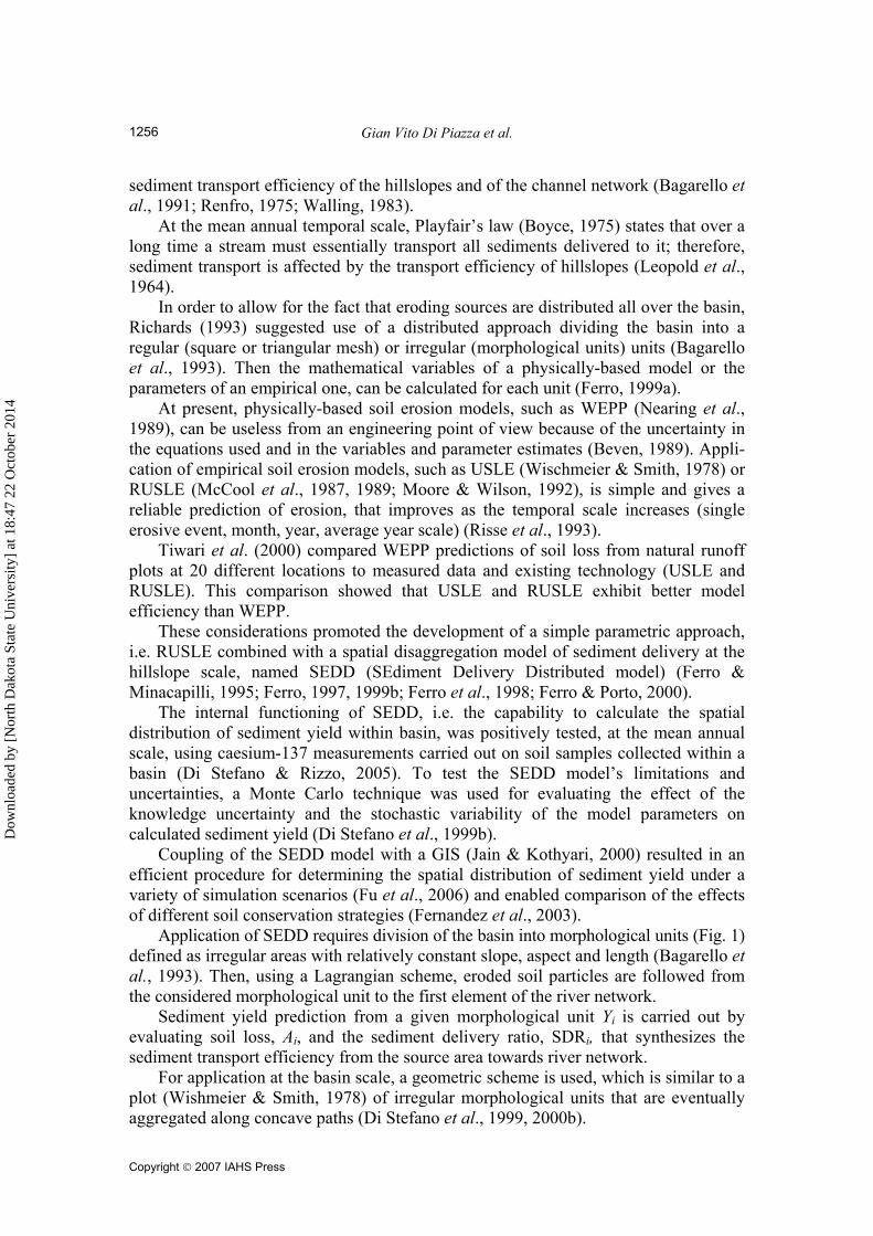
sediment transport efficiency of the hillslopes and of the channel network (Bagarello et al., 1991; Renfro, 1975; Walling, 1983). At the mean annual temporal scale, Playfair’s law (Boyce, 1975) states that over a long time a stream must essentially transport all sediments delivered to it; therefore, sediment transport is affected by the transport efficiency of hillslopes (Leopold et al., 1964). In order to allow for the fact that eroding sources are distributed all over the basin, Richards (1993) suggested use of a distributed approach dividing the basin into a regular (square or triangular mesh) or irregular (morphological units) units (Bagarello et al., 1993). Then the mathematical variables of a physically-based model or the parameters of an empirical one, can be calculated for each unit (Ferro, 1999a). At present, physically-based soil erosion models, such as WEPP (Nearing et al., 1989), can be useless from an engineering point of view because of the uncertainty in the equations used and in the variables and parameter estimates (Beven, 1989). Appli-cation of empirical soil erosion models, such as USLE (Wischmeier & Smith, 1978) or RUSLE (McCool et al., 1987, 1989; Moore & Wilson, 1992), is simple and gives a reliable prediction of erosion, that improves as the temporal scale increases (single erosive event, month, year, average year scale) (Risse et al., 1993). Tiwari et al. (2000) compared WEPP predictions of soil loss from natural runoff plots at 20 different locations to measured data and existing technology (USLE and RUSLE). This comparison showed that USLE and RUSLE exhibit better model efficiency than WEPP. These considerations promoted the development of a simple parametric approach, i.e. RUSLE combined with a spatial disaggregation model of sediment delivery at the hillslope scale, named SEDD (SEdiment Delivery Distributed model) (Ferro & Minacapilli, 1995; Ferro, 1997, 1999b; Ferro et al., 1998; Ferro & Porto, 2000). The internal functioning of SEDD, i.e. the capability to calculate the spatial distribution of sediment yield within basin, was positively tested, at the mean annual scale, using caesium-137 measurements carried out on soil samples collected within a basin (Di Stefano & Rizzo, 2005). To test the SEDD model’s limitations and uncertainties, a Monte Carlo technique was used for evaluating the effect of the knowledge uncertainty and the stochastic variability of the model parameters on calculated sediment yield (Di Stefano et al., 1999b). Coupling of the SEDD model with a GIS (Jain & Kothyari, 2000) resulted in an efficient procedure for determining the spatial distribution of sediment yield under a variety of simulation scenarios (Fu et al., 2006) and enabled comparison of the effects of different soil conservation strategies (Fernandez et al., 2003). Application of SEDD requires division of the basin into morphological units (Fig. 1) defined as irregular areas with relatively constant slope, aspect and length (Bagarello et al., 1993). Then, using a Lagrangian scheme, eroded soil particles are followed from the considered morphological unit to the first element of the river network. Sediment yield prediction from a given morphological unit Yi is carried out by evaluating soil loss, Ai, and the sediment delivery ratio, SDRi, that synthesizes the sediment transport efficiency from the source area towards river network. For application at the basin scale, a geometric scheme is used, which is similar to a plot (Wishmeier & Smith, 1978) of irregular morphological units that are eventually aggregated along concave paths (Di Stefano et al., 1999, 2000b).

Dow

nloa

ded

by [

Nor

th D

akot

a St

ate

Uni

vers

ity]

at 1

8:47

22

Oct

ober

201

4



1257

Fig. 1 Example of basin division into morphological units.

Morphological units are identified manually on the topographic map using Wischmeier’s (Wischmeier & Smith, 1965) definition of slope length and considering that each unit must have a constant slope and a single aspect. Use of data processing technologies, such as GIS, stimulated the use of a raster scheme according to which the studied area is divided into square cells of fixed mesh size, and their attributes are stored and elaborated using a matrix scheme. In order to respect the original Wischmeier model (Wischmeier & Smith, 1978), we used the subdivision into morphological unit and the ARC-INFO software raster scheme to produce the digital terrain model (DTM) and to calculate the mean slope for each morphological unit. Taking into account the hillslope component of the sediment delivery process, Ferro & Minacapilli (1995) suggested calculating the sediment delivery ratio SDRi of each morphological unit as:

( )⎟⎟

⎠

⎞

⎜⎜

⎝

⎛−=⎟

⎟

⎠

⎞

⎜⎜

⎝

⎛−=−= ∑

=

pN

j ji

ji

ip

ipipi s

λβ

s

lβtβ

1 ,

,

,

,, expexpexpSDR (1)

where β (m-1) is a coefficient; tp,i (m) is the travel time of the eroded particles from a given unit, i, to the first element of the river network; Np is the number of the morphological units located along the generic hydraulic path of length lp,i (m) and slope sp,i (m m-1); and λi,j (m) and si,j (m m-1) are, respectively, the length and slope of each morphological unit j located along the path from the morphological unit i to the first element of the river network. Sediment yield Yi (t) of the morphological unit i can be calculated by:

iuiiiiiii SPCKRY ,SDRLS= (2)

where Ri (t ha-1 per unit of soil erodibility, Ki) is the rainfall erosivity factor of the morphological unit i; Ki (t ha-1 per unit of soil erosivity, Ri) is the soil erodibility factor;

Dow

nloa

ded

by [

Nor

th D

akot

a St

ate

Uni

vers

ity]

at 1

8:47

22

Oct

ober

201

4



1258

Ci (dimensionless) is the cover and management factor; Pi (dimensionless) is the support practice factor; Su,i is the morphological unit area (ha); and LSi (dimensionless) is the topographic factor calculated using the expression proposed by McCool et al. (1987, 1989):

( )03.0sin8.1013.22

LS +⎟⎠⎞

⎜⎝⎛= i

mi

i αλ i

if tan αi ≤ 0.09 (3a)

( )5.0sin8.1613.22

LS −⎟⎠⎞

⎜⎝⎛= i

mi

i αλ i

if tan αi ≥ 0.09 (3b)

where λi (m) is the length of the morphological unit i, αi (radians) is the slope angle of the morphological unit i and mi is an exponent that has the following expression:

i

ii fa

fam

+=

1 (4)

where a is a coefficient, set to 1 following McCool et al. (1989) and Di Stefano et al. (2000a), while fi is expressed by the following relationship:

( )56.0sin30896.0sin

8.0 +=

i

ii α

αf (5)

The estimate of the coefficient β, appearing in (1), is carried out using the sediment balance equation establishing that basin sediment yield Ys (t) can be obtained by summing up the sediment yield of each morphological unit identified in the basin:

( ) iuiiiii

N

i

N

iipiuiiiiiis SPCKRtβSPCKRY

u u

,1 1

,, LSexpLSSDR∑ ∑= =

−== (6)

where Nu is the number of morphological units. Equation (6) led to the sediment delivery relationship, i.e. between the sediment delivery ratio of the whole basin SDRw and the same ratio of each morphological unit. Ferro & Minacapilli (1995) showed that this relationship does not depend on the erosion model and that it can be expressed by the following equation in which only morphological data appear:

( )

∑

∑

=

=

−=

u

u

N

iiuii

iuii

N

iip

w

Ssλ

Ssλtβ

1,

25.0

,25.0

1,exp

SDR (7)

When applying the SEDD model to large basins, relationship (7) is very useful to estimate coefficient β for a basin divided into morphological units if a measurement of SDRw is available (for example, from sediment transport measurements carried out at the basin outlet). For Sicilian basins of area between 20 and 70 km2, other studies (ASCE, 1975; Bagarello et al., 1991; Di Stefano et al., 2002) have established a relationship between SDRw and basin area S. This analysis, carried out for six Sicilian basins of area 20–70 km2 for which reservoir sedimentation data are available, allowed derivation of the equation:

Dow

nloa

ded

by [

Nor

th D

akot

a St

ate

Uni

vers

ity]

at 1

8:47

22

Oct

ober

201

4



1259

( )Sbw −= expSDR (8)

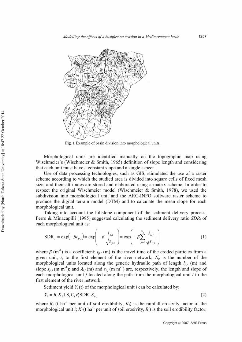
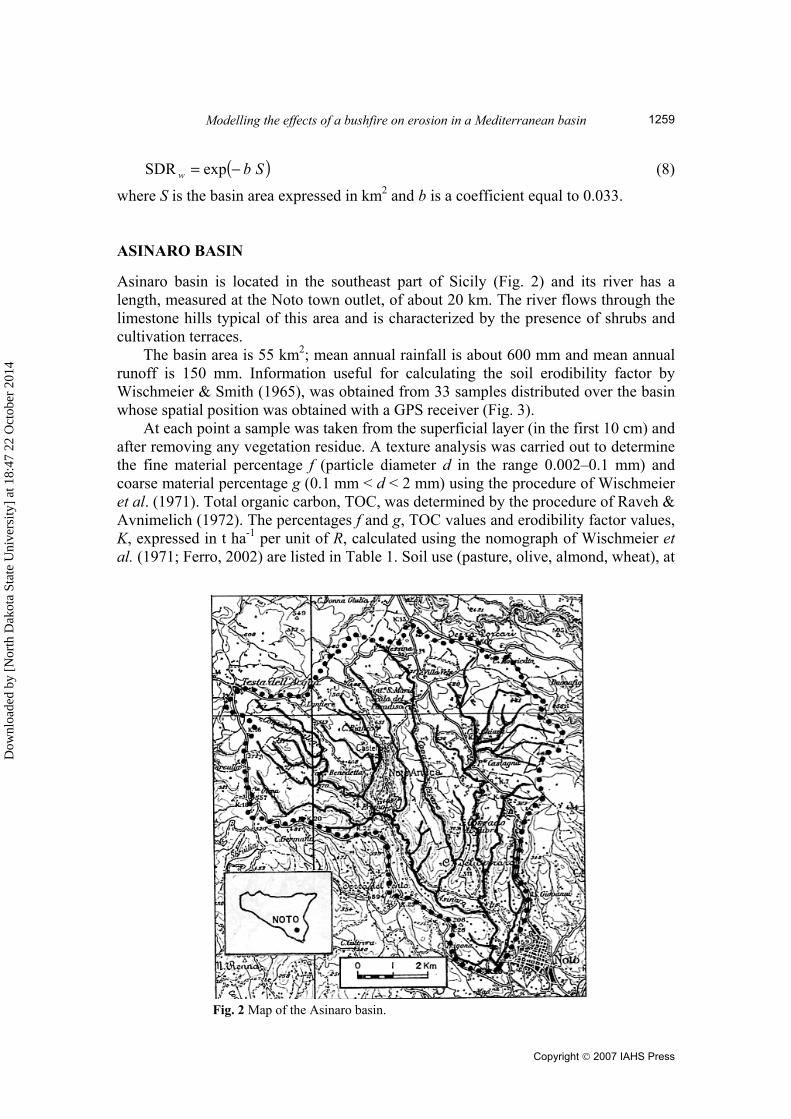
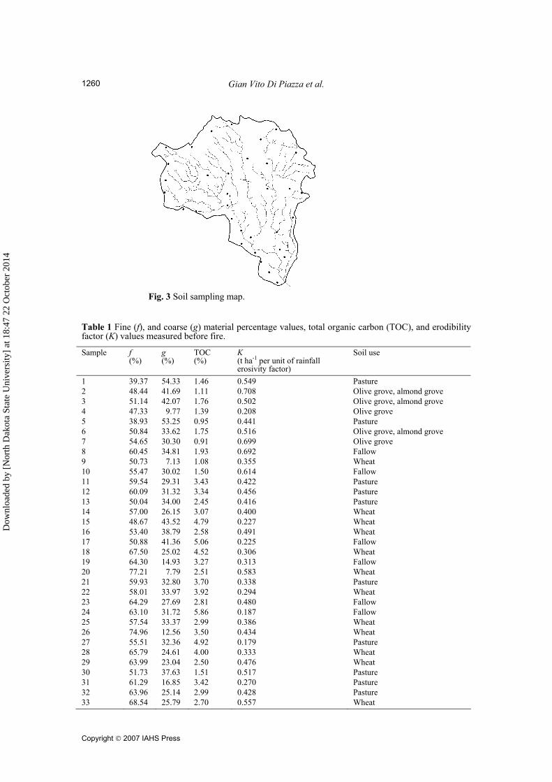
where S is the basin area expressed in km2 and b is a coefficient equal to 0.033. ASINARO BASIN Asinaro basin is located in the southeast part of Sicily (Fig. 2) and its river has a length, measured at the Noto town outlet, of about 20 km. The river flows through the limestone hills typical of this area and is characterized by the presence of shrubs and cultivation terraces. The basin area is 55 km2; mean annual rainfall is about 600 mm and mean annual runoff is 150 mm. Information useful for calculating the soil erodibility factor by Wischmeier & Smith (1965), was obtained from 33 samples distributed over the basin whose spatial position was obtained with a GPS receiver (Fig. 3). At each point a sample was taken from the superficial layer (in the first 10 cm) and after removing any vegetation residue. A texture analysis was carried out to determine the fine material percentage f (particle diameter d in the range 0.002–0.1 mm) and coarse material percentage g (0.1 mm < d < 2 mm) using the procedure of Wischmeier et al. (1971). Total organic carbon, TOC, was determined by the procedure of Raveh & Avnimelich (1972). The percentages f and g, TOC values and erodibility factor values, K, expressed in t ha-1 per unit of R, calculated using the nomograph of Wischmeier et al. (1971; Ferro, 2002) are listed in Table 1. Soil use (pasture, olive, almond, wheat), at

Fig. 2 Map of the Asinaro basin.

Dow

nloa

ded

by [

Nor

th D

akot

a St

ate

Uni

vers

ity]

at 1

8:47

22

Oct

ober

201

4



1260

Fig. 3 Soil sampling map.

Table 1 Fine (f), and coarse (g) material percentage values, total organic carbon (TOC), and erodibility factor (K) values measured before fire.

Sample f (%)

g (%)

TOC (%)

K (t ha-1 per unit of rainfall erosivity factor)

Soil use

1 39.37 54.33 1.46 0.549 Pasture 2 48.44 41.69 1.11 0.708 Olive grove, almond grove 3 51.14 42.07 1.76 0.502 Olive grove, almond grove 4 47.33 9.77 1.39 0.208 Olive grove 5 38.93 53.25 0.95 0.441 Pasture 6 50.84 33.62 1.75 0.516 Olive grove, almond grove 7 54.65 30.30 0.91 0.699 Olive grove 8 60.45 34.81 1.93 0.692 Fallow 9 50.73 7.13 1.08 0.355 Wheat 10 55.47 30.02 1.50 0.614 Fallow 11 59.54 29.31 3.43 0.422 Pasture 12 60.09 31.32 3.34 0.456 Pasture 13 50.04 34.00 2.45 0.416 Pasture 14 57.00 26.15 3.07 0.400 Wheat 15 48.67 43.52 4.79 0.227 Wheat 16 53.40 38.79 2.58 0.491 Wheat 17 50.88 41.36 5.06 0.225 Fallow 18 67.50 25.02 4.52 0.306 Wheat 19 64.30 14.93 3.27 0.313 Fallow 20 77.21 7.79 2.51 0.583 Wheat 21 59.93 32.80 3.70 0.338 Pasture 22 58.01 33.97 3.92 0.294 Wheat 23 64.29 27.69 2.81 0.480 Fallow 24 63.10 31.72 5.86 0.187 Fallow 25 57.54 33.37 2.99 0.386 Wheat 26 74.96 12.56 3.50 0.434 Wheat 27 55.51 32.36 4.92 0.179 Pasture 28 65.79 24.61 4.00 0.333 Wheat 29 63.99 23.04 2.50 0.476 Wheat 30 51.73 37.63 1.51 0.517 Pasture 31 61.29 16.85 3.42 0.270 Pasture 32 63.96 25.14 2.99 0.428 Pasture 33 68.54 25.79 2.70 0.557 Wheat

Dow

nloa

ded

by [

Nor

th D

akot

a St

ate

Uni

vers

ity]

at 1

8:47

22

Oct

ober

201

4



1261

the time of sampling, is also reported in Table 1. This soil use indication was used to classify soil use in the unburnt areas of the basin. The rainfall erosivity factor was calculated by the procedure of Bagarello & D’Asaro (1994) using daily rainfall data. In particular, the historical sequences corresponding to the periods 1973–1977, 1985–1988 and 1994–2000 of the raingauge at Noto were used for applying the procedure. The rainfall erosivity factor of each event, EIe, was calculated using the relationship (Bagarello & D’Asaro, 1994): EIe = αhe

γ (9) where he is the rainfall depth of the erosive event and α and γ are two coefficients that, for Noto station, equal 0.314 and 1.538 respectively (Bagarello & D’Asaro, 1994). Annual values of the rainfall factor Raj, listed in Table 2, were then calculated by summing the rainfall erosivity factor values of all events occurring in the year j. The mean annual value, for the period 1973–2000, is 72.6 t ha-1 per unit of K. In order to apply the SEDD model for three different scenarios after fire, the rainfall erosivity factor, RP, was calculated for the periods July–December 1998 (i.e. six months after fire), July 1998–July 1999 (one year after fire) and July 1998–July 2000 (two years after fire); the RP values are, respectively, 14.1, 17.3 and 241.7 t ha-1 per unit of K (Table 2). For calculating the topographic factors, using equation (3), the basin was divided in 854 morphological units that were digitized using the ARCInfo software. The digital terrain modelling (DTM) was carried out using a digitized contour line map (1:25 000 scale) and using the GRID module of ARCInfo with a mesh size of 50 m. The DTM permitted us to obtain the spatial distribution of slope and, so, calculate the mean slope of each morphological unit; this is a weighted mean (with area as weight) of the slope values of the square cells falling into the morphological unit. Images from two passes (27 June 1998 and 13 July 1998) of the Landsat TM satellite were used to carry out land-use mapping for before and after the passage of fire. Each image was classified using a supervised technique based both on ground control points, corresponding to each sample (Table 1), and on a map compiled by Table 2 Values of rainfall factor, measured at Noto station, at annual (Rai) and period (Rp) scale (t ha-1 per unit of erodibility factor).

Year Raj Period RP 1973 48.1 July–December 1998 14.1 1974 24.9 July 1998–July 1999 17.3 1975 77.9 July 1998–July 20000 241.7 1976 80.8 1977 42.8 1985 67.7 1986 105.2 1987 10.5 1988 29.0 1994 60.9 1995 62.9 1996 140.3 1997 130.2 1998 34.5 1999 167.2 2000 79.2

Dow

nloa

ded

by [

Nor

th D

akot

a St

ate

Uni

vers

ity]

at 1

8:47

22

Oct

ober

201

4



1262

wheat, pasture, seasonal horticultural crops mediterranean shrubs citrus grove olive grove, almond grove urban areas

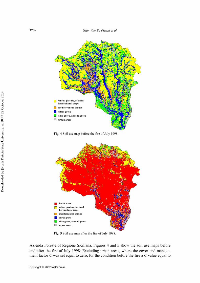
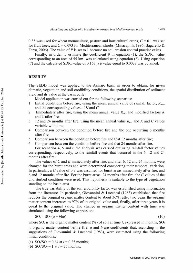
Fig. 4 Soil use map before the fire of July 1998.

burnt areas wheat, pasture, seasonal horticultural crops mediterranean shrubs citrus grove olive grove, almond grove urban areas

Fig. 5 Soil use map after the fire of July 1998.

Azienda Foreste of Regione Siciliana. Figures 4 and 5 show the soil use maps before

and after the fire of July 1998. Excluding urban areas, where the cover and manage-ment factor C was set equal to zero, for the condition before the fire a C value equal to

Dow

nloa

ded

by [

Nor

th D

akot

a St

ate

Uni

vers

ity]

at 1

8:47

22

Oct

ober

201

4



1263

0.35 was used for wheat monoculture, pasture and horticultural crops, C = 0.1 was set for fruit trees, and C = 0.093 for Mediterranean shrubs (Minacapilli, 1996; Bagarello & Ferro, 2006). The value of P is set to 1 because no soil erosion control practise exists. Finally, in order to estimate the coefficient β in equation (1), the SDRw value corresponding to an area of 55 km2 was calculated using equation (8). Using equation (7) and the calculated SDRw value of 0.163, a β value equal to 0.0038 was obtained. RESULTS The SEDD model was applied to the Asinaro basin in order to obtain, for given climatic, vegetation and soil erodibility conditions, the spatial distribution of sediment yield and its value at the basin outlet. Model application was carried out for the following scenarios: 1. Initial conditions before fire, using the mean annual value of rainfall factor, Rma,

and the corresponding values of K and C; 2. Immediately after fire, using the mean annual value Rma and modified factors K

and C after fire; 3. 12 and 24 months after fire, using the mean annual value Rma and K and C values

variable with time; 4. Comparison between the condition before fire and the one occurring 6 months

after fire; 5. Comparison between the condition before fire and that 12 months after fire; 6. Comparison between the condition before fire and that 24 months after fire. For scenarios 4, 5 and 6 the analysis was carried out using rainfall factor values corresponding, respectively, to the rainfall events that occurred in the 6, 12 and 24 months after fire. The values of C and K immediately after fire, and after 6, 12 and 24 months, were changed for the burnt areas and were determined considering their temporal variation. In particular, a C value of 0.9 was assumed for burnt areas immediately after fire, and 6 and 12 months after fire. For the burnt areas, 24 months after fire, the C values of the undisturbed condition were used. This hypothesis is suitable to the type of vegetation standing on the basin area. The true variability of the soil erodibility factor was established using information from the literature. In particular, Giovannini & Lucchesi (1983) established that fire reduces the original organic matter content to about 36%; after two years the organic matter content increases to 97% of its original value and, finally, after three years it is equal to the original value. The change in organic matter content with time was simulated using the following expression:

SOt = SOi (a + blnt) (10) where SOt is the organic matter content (%) of soil at time t, expressed in months, SOi

is organic matter content before fire, a and b are coefficients that, according to the suggestions of Giovannini & Lucchesi (1983), were estimated using the following initial conditions: (a) SOt/SOi = 0.64 at t = 0.25 months; (b) SOt/SOi = 1 at t = 36 months.

Dow

nloa

ded

by [

Nor

th D

akot

a St

ate

Uni

vers

ity]

at 1

8:47

22

Oct

ober

201

4



1264

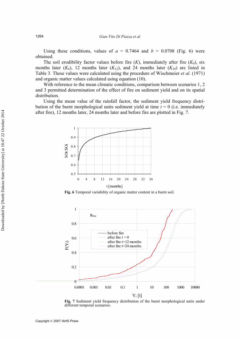
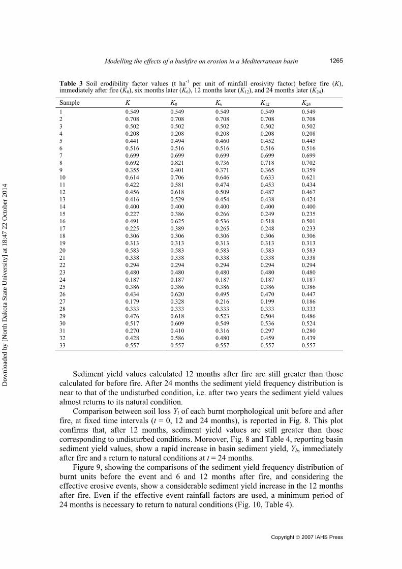
Using these conditions, values of a = 0.7464 and b = 0.0708 (Fig. 6) were obtained. The soil erodibility factor values before fire (K), immediately after fire (K0), six months later (K6), 12 months later (K12), and 24 months later (K24) are listed in Table 3. These values were calculated using the procedure of Wischmeier et al. (1971) and organic matter values calculated using equation (10). With reference to the mean climatic conditions, comparison between scenarios 1, 2 and 3 permitted determination of the effect of fire on sediment yield and on its spatial distribution. Using the mean value of the rainfall factor, the sediment yield frequency distri-bution of the burnt morphological units sediment yield at time t = 0 (i.e. immediately after fire), 12 months later, 24 months later and before fire are plotted in Fig. 7.

0.5

0.6

0.7

0.8

0.9

1

0 4 8 12 16 20 24 28 32 36

t [months]

SOt/S

Oi

Fig. 6 Temporal variability of organic matter content in a burnt soil.

0

0.2

0.4

0.6

0.8

1

0.0001 0.001 0.01 0.1 1 10 100 1000 10000

Yi [t]

F(Y

i)

before fireafter fire t = 0after fire t=12 monthsafter fire t=24 months

Rm,a

Fig. 7 Sediment yield frequency distribution of the burnt morphological units under different temporal scenarios.

Dow

nloa

ded

by [

Nor

th D

akot

a St

ate

Uni

vers

ity]

at 1

8:47

22

Oct

ober

201

4



1265

Table 3 Soil erodibility factor values (t ha-1 per unit of rainfall erosivity factor) before fire (K), immediately after fire (K0), six months later (K6), 12 months later (K12), and 24 months later (K24).

Sample K K0 K6 K12 K24 1 0.549 0.549 0.549 0.549 0.549 2 0.708 0.708 0.708 0.708 0.708 3 0.502 0.502 0.502 0.502 0.502 4 0.208 0.208 0.208 0.208 0.208 5 0.441 0.494 0.460 0.452 0.445 6 0.516 0.516 0.516 0.516 0.516 7 0.699 0.699 0.699 0.699 0.699 8 0.692 0.821 0.736 0.718 0.702 9 0.355 0.401 0.371 0.365 0.359 10 0.614 0.706 0.646 0.633 0.621 11 0.422 0.581 0.474 0.453 0.434 12 0.456 0.618 0.509 0.487 0.467 13 0.416 0.529 0.454 0.438 0.424 14 0.400 0.400 0.400 0.400 0.400 15 0.227 0.386 0.266 0.249 0.235 16 0.491 0.625 0.536 0.518 0.501 17 0.225 0.389 0.265 0.248 0.233 18 0.306 0.306 0.306 0.306 0.306 19 0.313 0.313 0.313 0.313 0.313 20 0.583 0.583 0.583 0.583 0.583 21 0.338 0.338 0.338 0.338 0.338 22 0.294 0.294 0.294 0.294 0.294 23 0.480 0.480 0.480 0.480 0.480 24 0.187 0.187 0.187 0.187 0.187 25 0.386 0.386 0.386 0.386 0.386 26 0.434 0.620 0.495 0.470 0.447 27 0.179 0.328 0.216 0.199 0.186 28 0.333 0.333 0.333 0.333 0.333 29 0.476 0.618 0.523 0.504 0.486 30 0.517 0.609 0.549 0.536 0.524 31 0.270 0.410 0.316 0.297 0.280 32 0.428 0.586 0.480 0.459 0.439 33 0.557 0.557 0.557 0.557 0.557

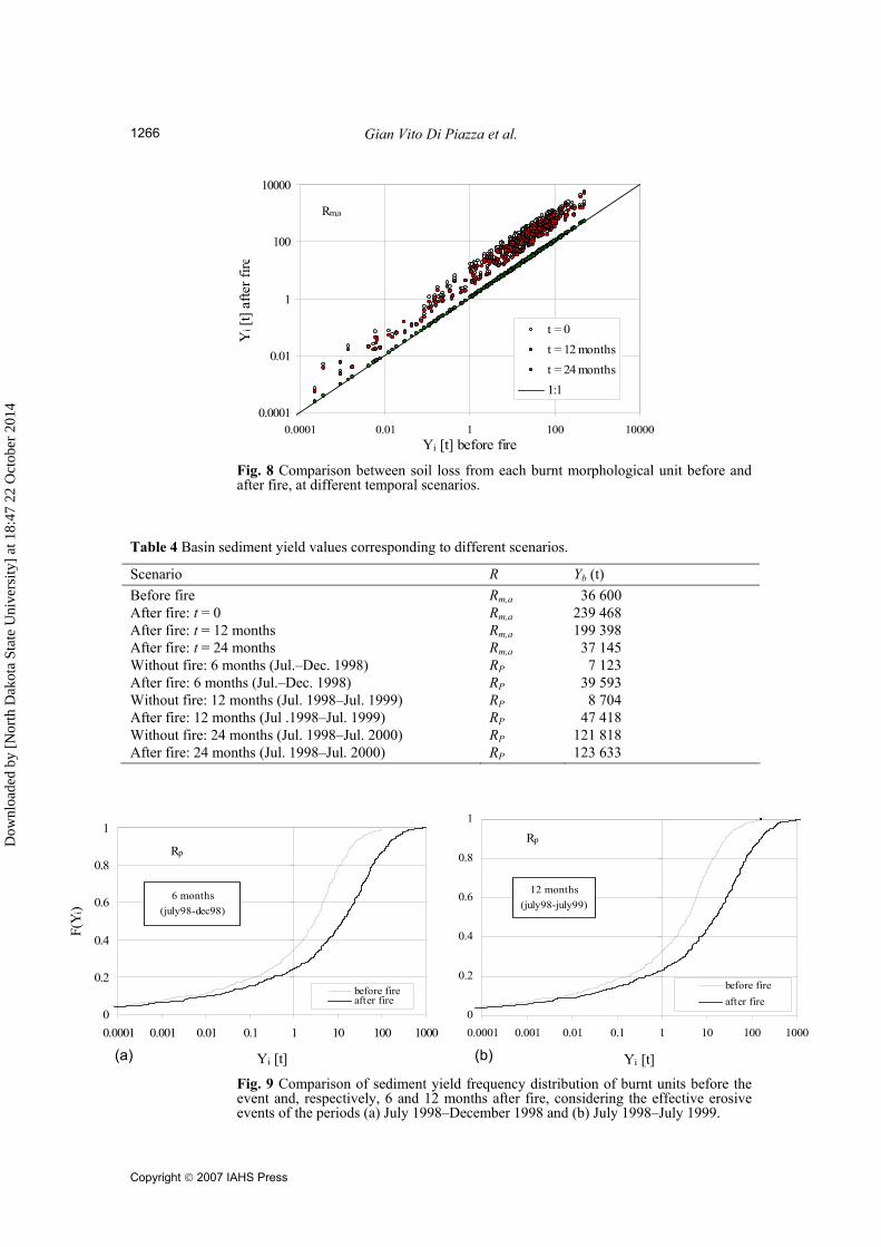
Sediment yield values calculated 12 months after fire are still greater than those calculated for before fire. After 24 months the sediment yield frequency distribution is near to that of the undisturbed condition, i.e. after two years the sediment yield values almost returns to its natural condition. Comparison between soil loss Yi of each burnt morphological unit before and after fire, at fixed time intervals (t = 0, 12 and 24 months), is reported in Fig. 8. This plot confirms that, after 12 months, sediment yield values are still greater than those corresponding to undisturbed conditions. Moreover, Fig. 8 and Table 4, reporting basin sediment yield values, show a rapid increase in basin sediment yield, Yb, immediately after fire and a return to natural conditions at t = 24 months. Figure 9, showing the comparisons of the sediment yield frequency distribution of burnt units before the event and 6 and 12 months after fire, and considering the effective erosive events, show a considerable sediment yield increase in the 12 months after fire. Even if the effective event rainfall factors are used, a minimum period of 24 months is necessary to return to natural conditions (Fig. 10, Table 4).

Dow

nloa

ded

by [

Nor

th D

akot

a St

ate

Uni

vers

ity]

at 1

8:47

22

Oct

ober

201

4



1266

0.0001

0.01

1

100

10000

0.0001 0.01 1 100 10000Yi [t] before fire

Yi [

t] af

ter f

ire

t = 0t = 12 monthst = 24 months1:1

Rm,a

Fig. 8 Comparison between soil loss from each burnt morphological unit before and after fire, at different temporal scenarios.

Table 4 Basin sediment yield values corresponding to different scenarios.

Scenario R Yb (t) Before fire Rm,a 36 600 After fire: t = 0 Rm,a 239 468 After fire: t = 12 months Rm,a 199 398 After fire: t = 24 months Rm,a 37 145 Without fire: 6 months (Jul.–Dec. 1998) RP 7 123 After fire: 6 months (Jul.–Dec. 1998) RP 39 593 Without fire: 12 months (Jul. 1998–Jul. 1999) RP 8 704 After fire: 12 months (Jul .1998–Jul. 1999) RP 47 418 Without fire: 24 months (Jul. 1998–Jul. 2000) RP 121 818 After fire: 24 months (Jul. 1998–Jul. 2000) RP 123 633

0

0.2

0.4

0.6

0.8

1

0.0001 0.001 0.01 0.1 1 10 100 1000

Yi [t]

F(Y

i)

before fireafter fire

Rp

6 months (july98-dec98)

0

0.2

0.4

0.6

0.8

1

0.0001 0.001 0.01 0.1 1 10 100 1000

Yi [t]


Rp

12 months(july98-july99)

Fig. 9 Comparison of sediment yield frequency distribution of burnt units before the event and, respectively, 6 and 12 months after fire, considering the effective erosive events of the periods (a) July 1998–December 1998 and (b) July 1998–July 1999.

(a) (b)

Dow

nloa

ded

by [

Nor

th D

akot

a St

ate

Uni

vers

ity]

at 1

8:47

22

Oct

ober

201

4



1267

0.0001

0.01

1

100

10000

0.0001 0.001 0.01 0.1 1 10 100 1000 10000

Yi [t] before fire

Yi [

t] af

ter f

ire

july 98 - december 98july 98 - july 99july 98 - july 001:1

Rp

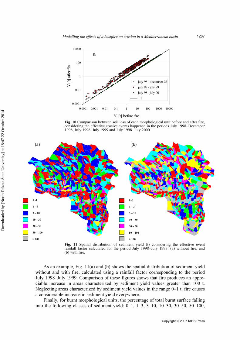
Fig. 10 Comparison between soil loss of each morphological unit before and after fire, considering the effective erosive events happened in the periods July 1998–December 1998, July 1998–July 1999 and July 1998–July 2000.

0 -1 1 – 3 3 – 10 10 – 30 30 – 50 50 – 100 > 100

0 -1 1 – 3 3 – 10 10 – 30 30 – 50 50 – 100 > 100

Fig. 11 Spatial distribution of sediment yield (t) considering the effective event rainfall factor calculated for the period July 1998–July 1999: (a) without fire, and (b) with fire.

As an example, Fig. 11(a) and (b) shows the spatial distribution of sediment yield without and with fire, calculated using a rainfall factor corresponding to the period July 1998–July 1999. Comparison of these figures shows that fire produces an appre-ciable increase in areas characterized by sediment yield values greater than 100 t. Neglecting areas characterized by sediment yield values in the range 0–1 t, fire causes a considerable increase in sediment yield everywhere. Finally, for burnt morphological units, the percentage of total burnt surface falling into the following classes of sediment yield: 0–1, 1–3, 3–10, 10–30, 30–50, 50–100,

(a) (b)

Dow

nloa

ded

by [

Nor

th D

akot

a St

ate

Uni

vers

ity]

at 1

8:47

22

Oct

ober

201

4



1268

0

0.1

0.2

0.3

0.4

0.5

0.6

0-1 1-3 3-10 10-30 30-50 50-100 >100

Y [t]

P(Y)


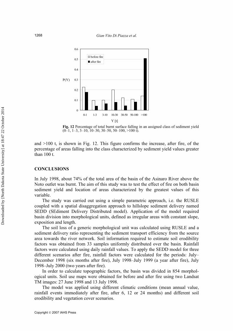
Fig. 12 Percentage of total burnt surface falling in an assigned class of sediment yield (0–1, 1–3, 3–10, 10–30, 30–50, 50–100, >100 t).

and >100 t, is shown in Fig. 12. This figure confirms the increase, after fire, of the percentage of areas falling into the class characterized by sediment yield values greater than 100 t. CONCLUSIONS In July 1998, about 74% of the total area of the basin of the Asinaro River above the Noto outlet was burnt. The aim of this study was to test the effect of fire on both basin sediment yield and location of areas characterized by the greatest values of this variable. The study was carried out using a simple parametric approach, i.e. the RUSLE coupled with a spatial disaggregation approach to hillslope sediment delivery named SEDD (SEdiment Delivery Distributed model). Application of the model required basin division into morphological units, defined as irregular areas with constant slope, exposition and length. The soil loss of a generic morphological unit was calculated using RUSLE and a sediment delivery ratio representing the sediment transport efficiency from the source area towards the river network. Soil information required to estimate soil erodibility factors was obtained from 33 samples uniformly distributed over the basin. Rainfall factors were calculated using daily rainfall values. To apply the SEDD model for three different scenarios after fire, rainfall factors were calculated for the periods: July–December 1998 (six months after fire), July 1998–July 1999 (a year after fire), July 1998–July 2000 (two years after fire). In order to calculate topographic factors, the basin was divided in 854 morphol-ogical units. Soil use maps were obtained for before and after fire using two Landsat TM images: 27 June 1998 and 13 July 1998. The model was applied using different climatic conditions (mean annual value, rainfall events immediately after fire, after 6, 12 or 24 months) and different soil erodibility and vegetation cover scenarios.

Dow

nloa

ded

by [

Nor

th D

akot

a St

ate

Uni

vers

ity]

at 1

8:47

22

Oct

ober

201

4



1269

The analysis carried out at the mean annual scale showed that 12 months after fire the sediment yield values are still greater than those of the undisturbed condition. In particular, sediment yield has a rapid increase in comparison to the undisturbed condi-tion immediately after fire and until 12 months after fire. According to the hypothesis made on the crop and management factor, it is only after 24 months that sediment yield values return to their initial values. Neglecting areas characterized by low sediment yield values, 0–1 t, the compari-son of sediment yield spatial distribution before and after fire shows an appreciable increase of sediment yield in each burnt morphological unit. Acknowledgements This research was carried out using a grant of Regione Siciliana – Assessorato Agricoltura e Foreste, Servizi allo Sviluppo – Progetto DESERTNET 2. C. Di Stefano and G. V. Di Piazza and V. Ferro contributed equally in setting up the research, applying the SEDD model and writing the paper. REFERENCES ASCE (1975) Sedimentation Engineering. ASCE Manuals & Reports on Engineering Practice no. 54, New York, USA. Bagarello, V. & D’Asaro, F. (1994) Estimating single storm erosion index. Trans. Am. Soc. Agric. Engrs 37(3), 785–791. Bagarello, V. & Ferro, V. (2006) Erosione e conservazione del suolo. McGraw-Hill, Milan, Italy. Bagarello, V., Ferro, V. & Giordano, G. (1991) Contributo alla valutazione del fattore di deflusso di Williams e del

coefficiente di resa solida per alcuni bacini idrografici siciliani. Rivista di Ingegneria Agraria 4, 238–251. Bagarello, V., Baiamonte, G., Ferro, V. & Giordano, G. (1993) Evaluating the topographic factors for watershed soil

erosion studies. In: Proc. Workshop on Soil Erosion in Semi-arid Mediterranean Areas (ed. by R. P. C. Morgan), 3–17. Taormina, Italy.

Beven, K. (1989) Changing ideas in hydrology—the case of physically-based models. J. Hydrol. 105, 157–172. Boyce, R. C. (1975) Sediment routing with sediment delivery ratios. In: Present and Prospective Technology for

Predicting Sediment Yield and Sources, 61–65. US Dept. Agric. Publ. ARS-S-40. Brown, J. A. H. (1972) Hydrologic effects of a brushfire in a catchment in southeastern New South Wales. J. Hydrol. 15, 77–96. Candela, A., Aronica , G. & Santoro, M. (2005) Effects of forest fires on flood frequency curves in a Mediterranean

catchment. Hydrol. Sci. J. 50(2), 193–206. DeBano, L. F. (2000) The role of fire and soil heating on water repellency in wildland environments: a review. J. Hydrol.

231–232, 195–206. DeBano, L. F., Mann, L. D. & Hamilton, D. A. (1970) Translocation of hydrophobic substances into soil by burning

organic litter. Soil Sci. Soc. Am. Proc. 34, 130–133. DeBano, L. F., Savage, S. M. & Hamilton, D. A. (1976) The transfer of heat and hydrophobic substances during burning.

Soil Sci. Soc. Am. Proc. 40, 779–782. Diaz-Fierros, F., Benito Rueda, E. & Perez Moreira, R. (1987) Evaluation of the USLE for the prediction of erosion on

burned forest areas in Galicia. Catena 14, 189–199. Di Stefano, C., Ferro, V. & Porto, P. (1999a) Modelling sediment delivery processes by a stream tube approach. Hydrol.

Sci. J. 44(5), 725–742. Di Stefano, C., Ferro, V. & Porto, P. (1999b) Linking sediment yield and caesium-137 spatial distribution at basin scale. J.

Agric. Engng Res. 74, 41–62. Di Stefano, C., Ferro, V. & Porto, P. (2000a) Length slope factors for applying the revised universal soil loss equation at

basin scale in southern Italy. J. Agric. Engng Res. 75(4), 349–364. Di Stefano, C., Ferro, V., Porto, P. & Tusa, G. (2000b) Slope curvature influence on soil erosion and deposition processes.

Water Resour. Res. 36(2), 607–617. Di Stefano, C., Ferro, V., Giordano, G. & Minacapilli, M. (2002) Calibrazione di un modello distribuito per la stima della

produzione di sedimenti in bacini di media estensione. Atti del Convegno “La gestione integrata dei bacini idrografici”. Quaderni di Idronomia Montana 22, 233–248.

Di Stefano, C. & Rizzo, S. (2005) Impiego della tecnica del cesio-137 per il monitoraggio dei processi erosivi nel bacino sperimentale SPA2. Quaderni di Idronomia Montana 24, 553–570.

Fernandez, C., Wu, J. Q., McCool, D. K. & Stöckle, C. O. (2003) Estimating water erosion and sediment yield with GIS, RUSLE, and SEDD. J. Soil Water Conserv. 58(3), 128–136.

Ferro, V. (1997) Further remarks on a distributed approach to sediment delivery. Hydrol. Sci. J. 42(5), 633–647. Ferro, V. (1999a) Problematiche inerenti la modellazione e la misura dell’erosione e della produzione di sedimenti. In: Atti

del Seminario AIIA “Monitoraggio e modellazione dei Processi Idrologici” (Palermo), 1–80.

Dow

nloa

ded

by [

Nor

th D

akot

a St

ate

Uni

vers

ity]

at 1

8:47

22

Oct

ober

201

4



1270

Ferro, V. (1999b) Modellistica matematica e verifica sperimentale dell’approccio distribuito dei processi di sediment delivery. In: Atti del Convegno “La gestione dell’erosione”, Quaderni di Idronomia Montana (Trento) 19/1, 19–30. Editoriale Nuova Bios.

Ferro, V. (2002) La sistemazione dei bacini idrografici. McGraw-Hill, Milano, Italy. Ferro, V. & Minacapilli, M. (1995) Sediment delivery processes at basin scale. Hydrol. Sci. J. 40(6), 703–717. Ferro, V. & Porto, P. (2000) A sediment delivery distributed (SEDD) model. J. Hydrol. Engng ASCE 5(4), 411–422. Ferro, V., Di Stefano, C., Giordano, G. & Rizzo, S. (1998) Sediment delivery processes and the spatial distribution of

caesium-137 in a small Sicilian basin. Hydrol. Processes 12, 701–711. Floyd, A. G. (1966) Effect of fire upon weed seeds in the wet sclerophill forests of northern NSW. Aust. J. Bot. 14,

243–247. Fu, G., Chen, S. & McCool, D. K. (2006) Modeling the impacts of no-till practice on soil erosion and sediment yield with

RUSLE, SEDD and ArcView GIS. Soil & Tillage Res. 85, 38–49. Giovannini, G. & Lucchesi, S. (1983) Effect of fire on hydrophobic and cementing subsurface soil aggregates. Soil. Sci.

136, 231–236. Giovannini, G., Lucchesi, S. & Giachetti, M. (1987) The natural evolution of a burned soil: a three-year investigation. Soil

Sci. 143, 220–226. Giovannini, G., Lucchesi, S. & Giachetti, M. (1988) Effect of heating on some physical and chemical parameters related to

soil aggregation and erodibility. Soil Sci. 146, 255–261. Inbar, M., Tamir, M. & Wittenberg, L. (1998) Runoff and erosion after a forest fire in Mount Carmel, a Mediterranean

area. Geomorphol. 24, 17–33. Jain, M. K. & Kothyari, U. C. (2000) Estimation of soil erosion and sediment yield using GIS. Hydrol. Sci. J. 45(5),

771–786. Lavee, H., Kutiel, P., Segev, M. & Benyamini, Y. (1995) Effect of roughness on runoff and erosion in a Mediterranean

ecosystem: the role of fire. Geomorphol. 11, 227–234. Leopold, L. B., Wolman, M. G. & Miller, J. P. (1964) Fluvial Processes in Geomorphology. W.H. Freeman and Co, San

Francisco, USA. McCool, D. K., Brown, L. C., Foster, G. R., Mutchler, C. K., Meyer, L. D. (1987) Revised slope steepness factor for the

universal soil loss equation. Trans. Am. Soc. Agric. Engrs 30(5), 1387–1396. McCool, D. K., Foster, G. R., Mutchler, C. K. & Meyer, L. D. (1989) Revised slope length factor for the Universal Soil

Loss Equation. Trans. Am. Soc. Agric. Engrs 32(5), 1571–1576. Minacapilli, M. (1996) Modelli matematici e GIS per la valutazione dell’erosione idrica nei bacini idrografici. Dottorato di

Ricerca in Idronomia Ambientale, VIII Ciclo, Dissertazione finale per il conseguimento del titolo, University of Palermo, Italy.

Moore, I. D. & Wilson, J. P. (1992) Length-slope factors for the revised universal soil loss equation: simplified methods of estimation. J. Soil Water Conserv. 47(5), 423–428.

Nearing, M. A., Foster, G. R., Lane, L. J. & Finkner, S. C. (1989) A process-based soil erosion model for USDA-Water Erosion Prediction Project Technology. Trans. Am. Soc. Agric. Engrs 32(5), 1587–1593.

Pimentel, D. (1993) World Soil Erosion and Conservation, Cambridge University Press, Cambridge, UK. Prosser, I. P. & Williams, L. (1998) The effect of wildfire on runoff and erosion in native Eucalyptus forest. Hydrol.

Processes 12, 251–265. Renfro, W. G. (1975) Use of erosion equation and sediment delivery ratios for predicting sediment yield. In: Present and

Prospective Technology for Predicting Sediment Yields and Sources, 33–45. US Dept Agric. Publ. ARS-S-40. Richards, K. (1993) Sediment delivery and drainage network. In: Channel Network Hydrology (ed. by K. Beven &

M. J. Kirkby), 221–254. John Wiley & Sons, Inc., New York, USA. Risse, L. M., Nearing, M. A., Nicks, A. & Laflen, J. M. (1993) Error assessment in the universal soil loss equation. Soil

Sci. Soc. Am. J. 57, 825–833. Rulli, M. C. (2000) Sulla valutazione della produzione di sedimenti da parte di un’area percorsa da incendio mediante un

approccio idrologico distribuito. Proc. Convegno Nazionale di Idraulica e Costruzioni Idrauliche IDRA, 2000, 109-117, Ed. Bios.

Savage, S. M., Osborn, J., Letey, J. & Heaton, C. (1972) Substances contributing to fire-induced water repellency in soils. Soil Sci. Soc. Am. Proc. 36, 674–678.

Soto, B. & Diaz-Fierros, F. (1998) Runoff and soil erosion from areas of burnt scrub : comparison of experimental results with those predicted by the WEPP model. Catena 31, 257–270.

Tiwari, A. K., Risse, L. M. & Nearing, M. A. (2000). Evaluation of WEPP and its comparison with USLE and RUSLE. Trans. Am. Soc. Agric. Engrs 43, 1129–1135.

Walling, D. E. (1983) The sediment delivery problem. J. Hydrol. 65, 209–237. Wischmeier, W. H. & Smith, D. D. (1965) Predicting Rainfall Erosion Losses from Cropland East of the Rocky

Mountains. US Dept Agric., Agric. Handbook 282, Washington, USA. Wischmeier, W. H. & Smith, D. D. (1978) Predicting Rainfall Erosion Losses. A Guide to Conservation Planning, US

Dept Agric., Agric. Handbook. Wischmeier, W. H., Johnson, C. D. & Cross, B. V. (1971) A soil erodibility nomograph for farmland and construction

sites. J. Soil Water Conserv. 29, 189–193. Received 10 May 2005; accepted 31 March 2007

Dow

nloa

ded

by [

Nor

th D

akot

a St

ate

Uni

vers

ity]

at 1

8:47

22

Oct

ober

201

4

Documents

Modelling the effects of a bushfire on erosion in a Mediterranean basin / Modélisation des impacts d'un incendie sur l'érosion dans un bassin Méditerranéen