Optical bullets and “rockets” in nonlinear dissipative systems and their transformations and interactions

Optical bullets and “rockets” in nonlinear dissipative systems and their transformations

and interactions. J. M. Soto-Crespo

Instituto de Optica, CSIC, Serrano 121, 28006 Madrid, Spain [email protected]

Philippe Grelu Laboratoire de Physique de l’Université de Bourgogne, Unité Mixte de Recherche 5027 du Centre National de

Recherche Scientifique, B.P. 47870, 21078 Dijon, France [email protected]

Nail Akhmediev Optical Sciences Group, Research School of Physical Sciences and Engineering, The Australian National

University, Canberra ACT 0200, Australia [email protected]

Abstract: We demonstrate the existence of stable optical light bullets in nonlinear dissipative media for both cases of normal and anomalous chromatic dispersion. The prediction is based on direct numerical simulations of the (3+1)-dimensional complex cubic-quintic Ginzburg-Landau equation. We do not impose conditions of spherical or cylindrical symmetry. Regions of existence of stable bullets are determined in the parameter space. Beyond the domain of parameters where stable bullets are found, unstable bullets can be transformed into “rockets” i.e. bullets elongated in the temporal domain. A few examples of the interaction between two optical bullets are considered using spatial and temporal interaction planes.

© 2006 Optical Society of America

OCIS codes: (060.5530) and (190.5530) Pulse propagation and solitons; (320.7110) Ultrafast nonlinear optics.

References and links

1. Y. Silberberg, “Collapse of optical pulses,” Opt. Lett. 15, 1282 (1990). 2. B. A. Malomed, D. Mihalache, F. Wise, and L. Torner, “Spatiotemporal solitons,” J. Opt. B. 7, R53 (2005). 3. N. N. Rosanov, “Spatial Hysteresis and Optical Patterns,” Springer, Berlin Heidelberg, 2002 (see section

6.6 and references therein); 4. N. Rosanov, “Solitons in laser systems with absorption,” chapter in “Dissipative solitons,” N. Akhmediev

and A. Ankiewicz eds., (Springer-Verlag, Berlin 2005). 5. Ph. Grelu, J. M. Soto-Crespo, and N. Akhmediev, “Light bullets and dynamic pattern formation in

nonlinear dissipative systems,” Opt. Express 13, 9352-9630 (2005). http://www.opticsinfobase.org/abstract.cfm?URI=oe-13-23-9352 6. C. Conti, S. Trillo, P. Di Trapani, G. Valiulis, A. Piskarskas, O. Jedrkiewicz, and J. Trull, “Nonlinear

Electromagnetic X Waves,” Phys. Rev. Lett., 90, 170406 (2003). 7. P. Di Trapani, G. Valiulis, A. Piskarskas, O. Jedrkiewicz, J. Trull, C. Conti and S. Trillo, “Spontaneously

generated X-shaped light bullets,” Phys. Rev. Lett., 91, 093904 (2003). 8. C. Zhou, M. Yu and X. He, “X-wave solutions of complex Ginzburg-Landau equations,” Phys. Rev. E 73,

026209 (2006). 9. M. Fermann, V. Kruglov, B. Thomsen, J. Dudley and J. Harvey, “Self-similar propagation and

amplification of parabolic pulses in optical fibers,” Phys. Rev. Lett., 84, 6010 (2000). 10. J. M. Soto-Crespo, N. N. Akhmediev, V. V. Afanasjev and S. Wabnitz, “Pulse solutions of the cubic-

quintic complex Ginzburg-Landau equation in the case of normal dispersion,” Phys. Rev E 55, 4783 (1997).

(C) 2006 OSA 1 May 2006 / Vol. 14, No. 9 / OPTICS EXPRESS 4013#68889 - $15.00 USD Received 14 March 2006; revised 13 April 2006; accepted 13 April 2006

mailto:[email protected]



http://www.opticsinfobase.org/abstract.cfm?URI=oe-13-23-9352

11. “Dissipative solitons,” edited by N. Akhmediev and A. Ankiewicz, (Springer-Verlag, Berlin 2005). 12. N. N. Akhmediev and A. Ankiewicz, “Solitons: nonlinear pulses and beams”, (Chapman & Hall, London,

1997).

1. Introduction

The search for stable propagation of confined wave packets is one of the major challenges in nonlinear optics. When nonlinearity provides stable confinement, the resultant wave packet is usually called a soliton. The term “optical bullet” was invented [1, 2] to depict a complete spatio-temporal soliton, for which confinement in the three spatial dimensions and localization in the temporal domain are achieved by the balance between a focusing nonlinearity and the spreading due to both chromatic dispersion and angular diffraction, while propagation in the medium takes place.

Recent theoretical advances have used the potential of nonlinear dissipation in order to find domains of existence for stable light bullets [3, 4]. Up to the present, these theoretical works have exclusively addressed the case of anomalous chromatic dispersion. Indeed, in paraxial models, anomalous dispersion and normalization generally allow to reduce the problem to the one with spherical symmetry in the propagation equation. Using spherical symmetry, the propagation equation can allow a tractable analytical approach [3]. As far as we know, the case of “bell-shaped” light bullets in normally dispersive media, when the variations in all three axes are independent, has not been addressed.

On the experimental side, it is important to stress that many interesting nonlinear materials feature normal chromatic dispersion in the wavelength domain of practical use. During the last few years, the study of propagation in normally dispersive media has attracted attention in several specific cases. Conti et al. [5] have shown that nonlinear conical waves, also called “X waves”, can be formed spontaneously together with nonlinear propagation in quadratic media that feature normal dispersion. These can lead to “X-shaped” light bullets in these particular media [6]. It is also possible that inhomogeneous media with specific properties be able to favor the formation of X-wave patterns, such as in the case of harmonic potential and particular boundary conditions as investigated theoretically in Ref. [7]. We can also mention the great interest for self-similar evolution of pulses in fibers that feature Kerr nonlinearity, gain and normal dispersion [8]. The latter situation corresponds to the formation of a self-similar temporal soliton; hence the terminology “similariton” has been applied. In fact, it was shown a few years ago that true bright temporal solitons in a normally dispersive medium can exist provided that nonlinear dissipation plays a key role [9]. These bright temporal solitons are examples of “dissipative solitons”, a field that has gained significant importance during recent years [10]. Exact analytical soliton solutions were found in the frame of the one-dimensional cubic-quintic complex Ginzburg-Landau equation (CCGLE), although all of them proved to be unstable. Numerical simulations allowed the finding of regions in the parameter space in which stable temporal solitons did exist. These stable solitons exhibited pulse shapes that could vary, from “bell-shaped” to “flat-top” temporal profiles, depending on the equation parameters [9].

Could these results be generalized to the three-dimensional CCGLE? The study undertaken by Rosanov [3] considered the generalized case of (m+1)D solitons with m=1,2 and 3 for the case of saturable nonlinearity with all three (spatial and time) variables normalized in a way which allows to deal with an equation which had spherical symmetry. The spatial and time variables cannot be completely equivalent. In particular, we relate the spectral filtering only to the retarded time variable and not to all three variables. Recently, we have numerically demonstrated the existence of stable, “bell-shaped”, light bullets using the three-dimensional CCGLE model in the case of anomalous dispersion. These can be called “dissipative light bullets” [4]. We showed that when a dissipative optical bullet exists for a given set of parameters, it possesses a finite basin of attraction.

In the present work, which is situated at the crossroad of [4] and [9], we explore, more systematically, a portion of the parameter space in which stable light bullets are found. We


find that dissipative light bullets also exist for the case of normal chromatic dispersion. In particular, we show that, for such media, bell-shaped profiles are found in both temporal and spatial transversal coordinates, in contrast to the conical shape of X-waves generated in quadratic normally dispersive media. Furthermore, we also show parameters for which the light bullet is not stable in the temporal domain, where its shape evolves towards a “rocket”. Additionally, we present some features of the interaction between stable dissipative optical bullets.

The rest of the paper is organized as follows. Section 2 presents the model and the numerical method used for solving the master equation. Section 3 is devoted to proving the existence of stable bullets for both normal and anomalous dispersions. Some regions of existence of stable optical bullets in the parameter space are shown. Examples of stable and unstable dissipative bullets are provided in Section 4. Section 5 deals with a special class of non-stationary solutions which we call “rockets”. The interaction between stable bullets is investigated in Section 6, while Section 7 contains our conclusions.

2. Model of the dissipative cubic-quintic medium

Our numerical simulations are based on an extended complex cubic-quintic Ginzburg-Landau equation (CCQGLE) model. This model, which is the same as that used in Ref. 4, includes cubic and quintic nonlinearities of dispersive and dissipative types, and we have added transverse operators to take spatial diffraction into account in the paraxial approximation. The normalized propagation equation reads:

iψz + D

2ψtt + 1

2ψxx + 1

2ψyy + ψ 2ψ+νψ 4ψ = iδψ+iεψ 2ψ+iβψtt +iμψ 4ψ . (1)

The optical envelope ψ is a function of four variables ψ = ψ (x,y,t,z), where t is the retarded time in the frame moving with the pulse, z is the propagation distance, and x and y are the two transverse coordinates. Equation (1) is written in normalized form. The left- hand-side of Eq. (1) contains the conservative terms, while all the terms responsible for gain or loss are on the right-hand-side. The parameter D accounts for dispersion. It is positive (negative) for the anomalous (normal) dispersion propagation regime. The parameter ν , if negative, is the saturation coefficient of the Kerr nonlinearity. In the following, the dispersion can take any value, and the saturation of the Kerr nonlinearity is kept relatively small in comparison with other parameters. As for the parameters δ, ε, β and μ , we note that δ is the coefficient for linear loss (if negative), ε is the nonlinear gain (if positive), β is spectral filtering (if positive) and μ is saturation of the nonlinear gain (if negative). In contrast to the model considered in Ref. 3, the spectral filtering only affects the term with the t variable, and the dispersion can have any sign. Furthermore, we do not introduce any symmetry constraints into our calculations. The variations of the envelope are thus independent along all axes.

This distributed model could be applied to the modeling of a wide-aperture laser cavity in the short pulse regime of operation. The model includes the effects of two-dimensional transverse diffraction of the beam, longitudinal dispersion of the pulse and its evolution along the cavity. Dissipative terms describe the gain and loss of the pulse in the cavity. Higher-order dissipative terms are responsible for the nonlinear transmission characteristics of the cavity, which allow, for example, passive mode-locking. This equation is a natural extension of the complex cubic-quintic Ginzburg-Landau equation (CCQGLE). We showed in Ref. 4 that, in the case of anomalous dispersion, this equation admits 3D dissipative solitons, i.e. optical bullets. In this paper, we show that they also exist for normal dispersion. Additionally, we study the regions of stable optical bullet existence in the parameter space, as well as the special behavior outside these regions where bullets become unstable.

We have solved Eq. (1) using a split-step Fourier method. Thus, the second-order derivative terms in x,y and t are solved in Fourier space. Consequently, we apply periodic boundary conditions in x, y and t. All other linear and nonlinear terms in the equation are solved in real space using a fourth-order Runge-Kutta method. The simulations presented in


the paper were performed using various grid sizes, ranging from 128 to 512 points in the three dimensions x, y and t. We have used various values of step sizes along the spatial and temporal domains to check that the results do not depend on the mesh intervals, thus avoiding any numerical artifact. Usually dz is taken to be 0.005. A typical numerical run lasts from several hours to several days on an up-to-date standard PC.

In the case of the (1+1)D CCQGLE, the equation admits soliton solutions [9]. Moreover, several solutions can co-exist for the same set of parameters. These solitons are not necessarily stable. Stability is controlled by the parameters of the equation and by the choice of the soliton branch. Stable and unstable optical bullets do exist in the case of (3+1)D simulations with equation (1) as well [4].

3. Regions of existence of optical bullets

Optical bullets exist in some regions in the parameter space. Clearly, it is difficult to find these regions in the 6-dimensional parameter space in which we operate. To begin with, we restrict ourselves to varying just two parameters, while fixing the other four. We have chosen the dispersion D and the cubic gain as the variable parameters. With β positive, it is possible to renormalize the time variable in Eq. (1) in such a way that the relevant parameter is simply D/β. This effectively reduces the dimension of the parameter space to 5. We view the dispersion coefficient D and the nonlinear gain coefficient ε as the main parameters that can be easily changed in most experiments with passively mode-locked lasers.

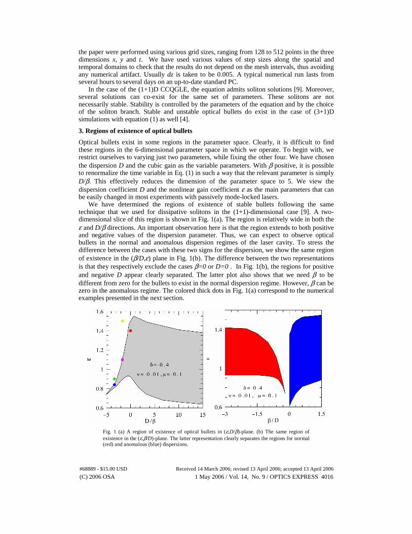
We have determined the regions of existence of stable bullets following the same technique that we used for dissipative solitons in the (1+1)-dimensional case [9]. A two- dimensional slice of this region is shown in Fig. 1(a). The region is relatively wide in both the ε and D/β directions. An important observation here is that the region extends to both positive and negative values of the dispersion parameter. Thus, we can expect to observe optical bullets in the normal and anomalous dispersion regimes of the laser cavity. To stress the difference between the cases with these two signs for the dispersion, we show the same region of existence in the (β/D,ε) plane in Fig. 1(b). The difference between the two representations is that they respectively exclude the cases β=0 or D=0 . In Fig. 1(b), the regions for positive and negative D appear clearly separated. The latter plot also shows that we need β to be different from zero for the bullets to exist in the normal dispersion regime. However, β can be zero in the anomalous regime. The colored thick dots in Fig. 1(a) correspond to the numerical examples presented in the next section.

Fig. 1 (a) A region of existence of optical bullets in (ε,D/β)-plane. (b) The same region of existence in the (ε,β/D)-plane. The latter representation clearly separates the regions for normal (red) and anomalous (blue) dispersions.


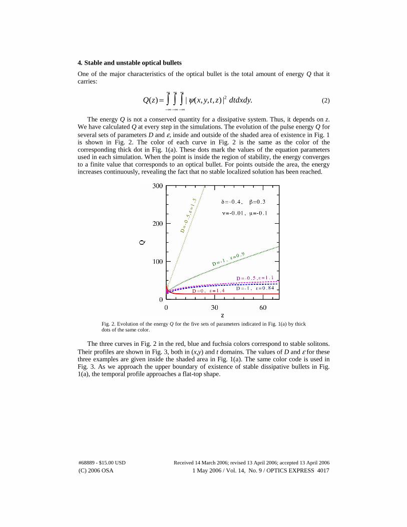
4. Stable and unstable optical bullets

One of the major characteristics of the optical bullet is the total amount of energy Q that it carries:

Q(z) = | ψ(x, y,t, z)−∞

∞

∫−∞

∞

∫−∞

∞

∫ |2 dtdxdy. (2)

The energy Q is not a conserved quantity for a dissipative system. Thus, it depends on z. We have calculated Q at every step in the simulations. The evolution of the pulse energy Q for several sets of parameters D and ε, inside and outside of the shaded area of existence in Fig. 1 is shown in Fig. 2. The color of each curve in Fig. 2 is the same as the color of the corresponding thick dot in Fig. 1(a). These dots mark the values of the equation parameters used in each simulation. When the point is inside the region of stability, the energy converges to a finite value that corresponds to an optical bullet. For points outside the area, the energy increases continuously, revealing the fact that no stable localized solution has been reached.

Fig. 2. Evolution of the energy Q for the five sets of parameters indicated in Fig. 1(a) by thick dots of the same color.

The three curves in Fig. 2 in the red, blue and fuchsia colors correspond to stable solitons.

Their profiles are shown in Fig. 3, both in (x,y) and t domains. The values of D and ε for these three examples are given inside the shaded area in Fig. 1(a). The same color code is used in Fig. 3. As we approach the upper boundary of existence of stable dissipative bullets in Fig. 1(a), the temporal profile approaches a flat-top shape.


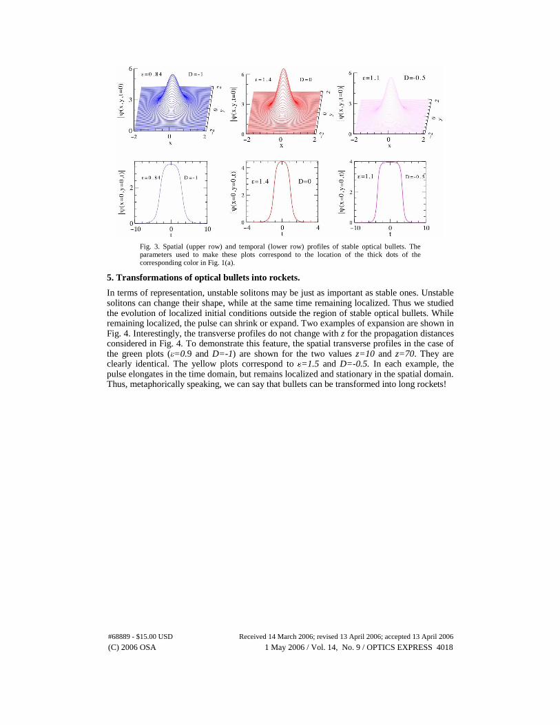
Fig. 3. Spatial (upper row) and temporal (lower row) profiles of stable optical bullets. The parameters used to make these plots correspond to the location of the thick dots of the corresponding color in Fig. 1(a).

5. Transformations of optical bullets into rockets.

In terms of representation, unstable solitons may be just as important as stable ones. Unstable solitons can change their shape, while at the same time remaining localized. Thus we studied the evolution of localized initial conditions outside the region of stable optical bullets. While remaining localized, the pulse can shrink or expand. Two examples of expansion are shown in Fig. 4. Interestingly, the transverse profiles do not change with z for the propagation distances considered in Fig. 4. To demonstrate this feature, the spatial transverse profiles in the case of the green plots (ε=0.9 and D=-1) are shown for the two values z=10 and z=70. They are clearly identical. The yellow plots correspond to ε=1.5 and D=-0.5. In each example, the pulse elongates in the time domain, but remains localized and stationary in the spatial domain. Thus, metaphorically speaking, we can say that bullets can be transformed into long rockets!


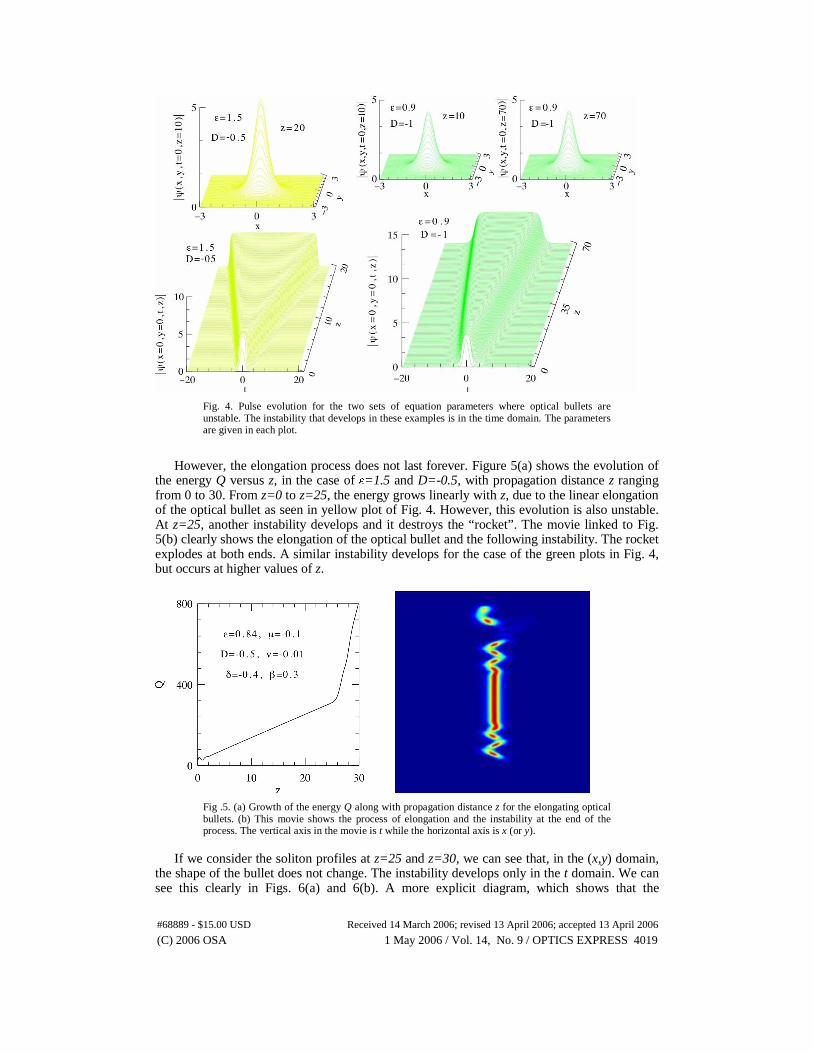
Fig. 4. Pulse evolution for the two sets of equation parameters where optical bullets are unstable. The instability that develops in these examples is in the time domain. The parameters are given in each plot.

However, the elongation process does not last forever. Figure 5(a) shows the evolution of the energy Q versus z, in the case of ε=1.5 and D=-0.5, with propagation distance z ranging from 0 to 30. From z=0 to z=25, the energy grows linearly with z, due to the linear elongation of the optical bullet as seen in yellow plot of Fig. 4. However, this evolution is also unstable. At z=25, another instability develops and it destroys the “rocket”. The movie linked to Fig. 5(b) clearly shows the elongation of the optical bullet and the following instability. The rocket explodes at both ends. A similar instability develops for the case of the green plots in Fig. 4, but occurs at higher values of z.

Fig .5. (a) Growth of the energy Q along with propagation distance z for the elongating optical bullets. (b) This movie shows the process of elongation and the instability at the end of the process. The vertical axis in the movie is t while the horizontal axis is x (or y).

If we consider the soliton profiles at z=25 and z=30, we can see that, in the (x,y) domain,

the shape of the bullet does not change. The instability develops only in the t domain. We can see this clearly in Figs. 6(a) and 6(b). A more explicit diagram, which shows that the


http://www.opticsexpress.org/viewmedia.cfm?id=89606&seq=1

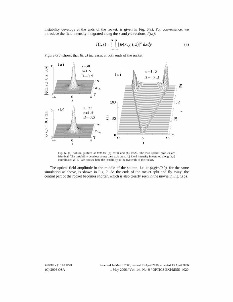
instability develops at the ends of the rocket, is given in Fig. 6(c). For convenience, we introduce the field intensity integrated along the x and y directions, I(t,z):

I(t, z) = | ψ−∞

∞

∫−∞

∞

∫ (x, y, t, z) |2 dxdy (3)

Figure 6(c) shows that I(t, z) increases at both ends of the rocket.

Fig. 6. (a) Soliton profiles at t=0 for (a) z=30 and (b) z=25. The two spatial profiles are identical. The instability develops along the t axis only. (c) Field intensity integrated along (x,y) coordinates vs. z. We can see here the instability at the two ends of the rocket.

The optical field amplitude in the middle of the soliton, i.e. at (x,y)=(0,0), for the same

simulation as above, is shown in Fig. 7. As the ends of the rocket split and fly away, the central part of the rocket becomes shorter, which is also clearly seen in the movie in Fig. 5(b).


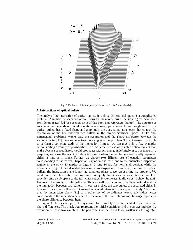
Fig. 7. Evolution of the temporal profile of the “rocket” at (x,y)=(0,0).

6. Interactions of optical bullets

The study of the interaction of optical bullets in a three-dimensional space is a complicated problem. A number of scenarios of collisions for the anomalous dispersion regime have been considered in Ref. [3] (see section 6.6.3 of this book and references therein). The outcome of an interaction depends on initial conditions and many parameters. Even though each of the optical bullets has a fixed shape and amplitude, there are some parameters that control the orientation of the line between two bullets in the three-dimensional space. Unlike one-dimensional problems, where only the separation and the phase difference between the solitons matter [11], now we have two more angles in the problem. Thus, it seems impossible to perform a complete study of the interaction. Instead, we can give only a few examples demonstrating a variety of possibilities. For each case, we use only stable optical bullets that, in the absence of a collision, would propagate without change indefinitely in z. For illustrative purposes, we show the result of interactions only when the two bullets are initially separated either in time or in space. Further, we choose two different sets of equation parameters corresponding to the normal dispersion regime in one case, and to the anomalous dispersion regime in the other. Examples in Figs. 8, 9, and 10 are for normal dispersion, while the example in Fig. 11 is calculated for anomalous dispersion. Clearly, in the case of optical bullets, the interaction plane is not the complete phase space representing the problem. We need more variables to show the trajectories uniquely. In this case, using an interaction plane provides only a sub-space of the full phase space. Nevertheless, it allows us to show the main features in the problem of the collision. Thus we will use the interaction plane method to show the interaction between two bullets. In our case, since the two bullets are separated either in time or in space, we will refer to temporal or spatial interaction planes, accordingly. We recall that the interaction plane [11] is a polar set of co-ordinates where the radius-vector corresponds to the separation between the maxima of the two solitons and the angle represents the phase difference between them.

Figure 8 shows examples of trajectories for a variety of initial spatial separations and phase differences. The black dots represent the initial conditions and the arrows indicate the evolution of these two variables. The parameters of the CCGLE are written inside Fig. 8(a).


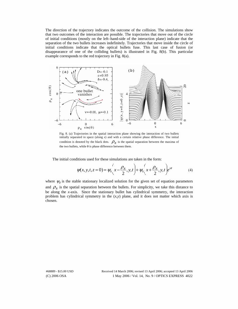
The direction of the trajectory indicates the outcome of the collision. The simulations show that two outcomes of the interaction are possible. The trajectories that move out of the circle of initial conditions (mostly on the left–hand-side of the interaction plane) indicate that the separation of the two bullets increases indefinitely. Trajectories that move inside the circle of initial conditions indicate that the optical bullets fuse. This last case of fusion (or disappearance of one of the colliding bullets) is illustrated in Fig. 8(b). This particular example corresponds to the red trajectory in Fig. 8(a).

Fig. 8. (a) Trajectories in the spatial interaction plane showing the interaction of two bullets initially separated in space (along x) and with a certain relative phase difference. The initial

condition is denoted by the black dots. ρR is the spatial separation between the maxima of

the two bullets, while θ is phase difference between them.

The initial conditions used for these simulations are taken in the form:

ψ(x, y,t, z = 0) = ψ0 x − ρR

2, y,t

⎛ ⎝ ⎜

⎞ ⎠ ⎟ + ψ0 x + ρR

2, y,t

⎛ ⎝ ⎜

⎞ ⎠ ⎟ eiθ (4)

where ψ0 is the stable stationary localized solution for the given set of equation parameters

and ρR is the spatial separation between the bullets. For simplicity, we take this distance to be along the x-axis. Since the stationary bullet has cylindrical symmetry, the interaction problem has cylindrical symmetry in the (x,y) plane, and it does not matter which axis is chosen.


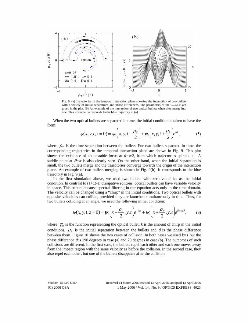
Fig. 9. (a) Trajectories in the temporal interaction plane showing the interaction of two bullets with a variety of initial separations and phase differences. The parameters of the CCGLE are given in the plot. (b) An example of the interaction of two optical bullets when they merge into one. This example corresponds to the blue trajectory in (a).

When the two optical bullets are separated in time, the initial condition is taken to have the

form:

ψ(x, y,t, z = 0) = ψ0 x, y,t − ρT

2

⎛ ⎝ ⎜

⎞ ⎠ ⎟ + ψ0 x, y,t + ρT

2

⎛ ⎝ ⎜

⎞ ⎠ ⎟ eiθ , (5)

where ρT is the time separation between the bullets. For two bullets separated in time, the corresponding trajectories in the temporal interaction plane are shown in Fig. 9. This plot shows the existence of an unstable focus at θ=π/2, from which trajectories spiral out. A saddle point at θ=π is also clearly seen. On the other hand, when the initial separation is small, the two bullets merge and the trajectories converge towards the origin of the interaction plane. An example of two bullets merging is shown in Fig. 9(b). It corresponds to the blue trajectory in Fig. 9(a).

In the first simulation above, we used two bullets with zero velocities as the initial condition. In contrast to (1+1)-D dissipative solitons, optical bullets can have variable velocity in space. This occurs because spectral filtering in our equation acts only in the time domain. The velocity can be changed using a “chirp” in the initial conditions. Two optical bullets with opposite velocities can collide, provided they are launched simultaneously in time. Thus, for two bullets colliding at an angle, we used the following initial condition:

ψ(x, y,t, z = 0) = ψ0 x − ρR

2, y,t

⎛ ⎝ ⎜

⎞ ⎠ ⎟ e−ikx +ψ0 x + ρR

2, y,t

⎛ ⎝ ⎜

⎞ ⎠ ⎟ eikx+iθ , (6)

where ψ0 is the function representing the optical bullet, k is the amount of chirp in the initial conditions, ρR is the initial separation between the bullets and θ is the phase difference between them. Figure 10 shows the two cases of collision. In both cases we used k=1 but the phase difference θ is 190 degrees in case (a) and 70 degrees in case (b). The outcomes of such collisions are different. In the first case, the bullets repel each other and each one moves away from the impact region with the same velocity as before the collision. In the second case, they also repel each other, but one of the bullets disappears after the collision.


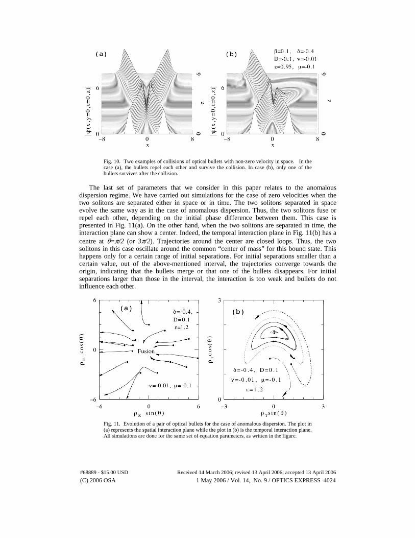
Fig. 10. Two examples of collisions of optical bullets with non-zero velocity in space. In the case (a), the bullets repel each other and survive the collision. In case (b), only one of the bullets survives after the collision.

The last set of parameters that we consider in this paper relates to the anomalous

dispersion regime. We have carried out simulations for the case of zero velocities when the two solitons are separated either in space or in time. The two solitons separated in space evolve the same way as in the case of anomalous dispersion. Thus, the two solitons fuse or repel each other, depending on the initial phase difference between them. This case is presented in Fig. 11(a). On the other hand, when the two solitons are separated in time, the interaction plane can show a center. Indeed, the temporal interaction plane in Fig. 11(b) has a centre at θ=π/2 (or 3π/2). Trajectories around the center are closed loops. Thus, the two solitons in this case oscillate around the common “center of mass” for this bound state. This happens only for a certain range of initial separations. For initial separations smaller than a certain value, out of the above-mentioned interval, the trajectories converge towards the origin, indicating that the bullets merge or that one of the bullets disappears. For initial separations larger than those in the interval, the interaction is too weak and bullets do not influence each other.

Fig. 11. Evolution of a pair of optical bullets for the case of anomalous dispersion. The plot in (a) represents the spatial interaction plane while the plot in (b) is the temporal interaction plane. All simulations are done for the same set of equation parameters, as written in the figure.


Numerical simulations for optical bullets are tedious and time consuming. Therefore, we stress again that no systematic studies can be done at this stage. Here we have given a few examples that, in no way, can be viewed as a complete investigation. The aim of presenting these examples is to demonstrate the wide variety of possibilities that occur in the collisions of optical bullets.

7. Conclusion

In conclusion, based on numerical simulations, we presented regions of existence of stable stationary optical bullets in a dissipative medium described by the 3-D complex cubic-quintic Ginzburg-Landau equation with an asymmetry between space and time variables. As far as we know, stable bell-shaped optical bullets were obtained for the first time in the normal region of chromatic dispersion, which is an important result with respect to existing nonlinear materials. The existence of bell-shaped optical bullets demonstrated here in the normal dispersion regime arises from the significance of nonlinear dissipation, in terms of magnitude as well as in terms of signs of all dissipative terms involved in the Ginzburg-Landau equation, whose physical meanings were given. In such conditions, localization can take place in the form of bell-shaped bullets, overcoming limitation from the sign of chromatic dispersion. Outside the regions of stable bullets, we observed a type of instability of the optical bullets that transforms them into “rockets”. Finally, examples of the interaction between stable optical bullets were presented using the temporal and spatial interaction planes, in the cases of either normal or anomalous chromatic dispersion.

Acknowledgments

The work of J. M. S. C. was supported by the M. E. y C. under contract BFM2003-00427. Ph. G. acknowledges support from Agence Nationale de la Recherche, and N. A. acknowledges support from the Australian Research Council. The authors are grateful to Dr. Ankiewicz for a critical reading of the manuscript.


Documents

Optical bullets and “rockets” in nonlinear dissipative systems and their transformations and interactions