Positive Mathematical Programming with Multiple Data ...ageconsearch.umn.edu/record/206148/files/CESR-57-27-50.pdf · programming models with a multi-commodity market model in an

Cahiers d’économie et sociologie rurales, n° 57, 2000

Positive MathematicalProgramming with Multiple

Data Points: A Cross-SectionalEstimation Procedure

Thomas HECKELEIWolfgang BRITZ

Thomas HECKELEI*, Wolfgang BRITZ*

Résumé – Cet article présente une approche visant à spécifier des fonctions de coûtnon linéaires dans le cadre de modèles de programmation régionaux. La méthodo-logie en question peut être considérée comme une application de la programmationmathématique positive (PMP) à des observations multiples. L’application de la PMPdans les modèles d’offre des produits agricoles s’est sensiblement développée aucours de ces dix dernières années. Cependant, beaucoup de modélisateurs n’ont pasfait état du comportement arbitraire et potentiellement invraisemblable des mo-dèles résultant de l’application standard de l’approche PMP. Paris et Howitt (1998)interprètent la PMP comme étant l’estimation d’une fonction de coût non linéaire etgénéralisent sa spécification en utilisant un procédé de «maximisation de l’entro-pie». Néanmoins, leur approche manque d’une base empirique suffisante. Elle com-porte toujours une paramétrisation nécessaire pour imposer les bonnes conditions decoubure de la fonction de coût, ce qui pose d’importants problèmes dans les appli-cations. La méthodologie que nous proposons est conçue pour exploiter l’informa-tion contenue dans un échantillon de données en coupes pour spécifier des fonctionsde coût quadratiques régionales avec des effets croisés entre les activités. L’approche apporte également une solution au problème de la courbure de la fonction de coût.Elle est appliquée ici à des modèles de programmation régionaux sur 22 régionsfrançaises. Une simulation a posteriori de la réforme de la Politique agricole com-mune de 1992 produit des résultats plausibles. Des prolongements de cette méthodeainsi que des améliorations possibles sont également identifiés.

Summary – This paper introduces an approach to the specification of non-linear cost func-tions in regional programming models. It can be characterised as an application of po-sitive mathematical programming (PMP) to multiple observations. The application ofPMP in policy relevant agricultural supply models as a mean for calibration has si-gnificantly increased during the last ten years. However, many modellers have not re-flected the arbitrary and potentially implausible response behaviour of the resulting mo-dels implied by standard applications of the approach. Paris and Howitt (1998)interpret PMP as the estimation of a non-linear cost function and generalize the speci-fication by employing a « Maximum Entropy (ME) » procedure. However, their ap-proach still lacks a sufficient empirical base and involves a parameterisation to enforcecorrect curvature of the cost function, which induces significant problems in applications.The suggested methodology is designed to exploit information contained in a cross sectio-nal sample to specify — regionally specific — quadratic cost functions with cross effectsfor crop activities. It also provides a solution to the curvature problem. The approach isapplied to regional programming models for 22 regions in France. An ex-post simula-tion across the 1992 CAP-reform shows plausible results with respect to the simulationbehaviour of the resulting models. Paths for extensions and improvements of this metho-dology are identified.

* Institute of Agricultural Policy, Market Research and Economic Sociology, Univer-sity of Bonn, Nussallee 21, 53115 Bonn, Germany.e-mail : [email protected] ; [email protected]

This research was pursued within the project « Common Agricultural Policy Regio-nal Impact» (CAPRI) which was partly funded under the FAIR program of the Eu-ropean Commission. The paper considerably benefited from the comments of twoanonymous referees and a co-editor. Even their extensive and constructive input probably left numerous errors for which the authors assume full responsability.

28

PositiveMathematicalProgramming withMultiple DataPoints :A Cross-SectionalEstimationProcedure

Key-words :positive mathematicalprogramming, maximumentropy estimation, curvature restrictions,ex-post validation

Programmationmathématique positiveavec observationsmultiples :estimationen coupestransversales

Mots-clés :programmationmathématique positive,méthode du maximumd’entropie, validation a posteriori, courbure de la fonction de coût

29

(1) For detailed information on the CAPRI project, consult Heckelei and Britz(2001) or the internet page http://www.agp.uni-bonn.de/agpo/rsrch/capri/capri_e. htm.

(2) Statistical Office of the European Communities.(3) The CAPRI database is currently updated until the year 2000. Complete-

ness at this point, however, is only guaranteed until 1995.

THE project «Common Agricultural Policy Regional Impact »(CAPRI) aims at regionally differentiated EU-wide analysis of

the CAP (1). The concept of the underlying comparative static modellingsystem combines a supply component comprising about 200 regionalprogramming models with a multi-commodity market model in an ite-rative fashion to endogenously determine regional supply and nationaldemand quantities, net trade at Member State and EU-level, and equili-brium market prices. The basic question that initiated the research pre-sented in this article is how to specify the regional programming modelssuch that they offer an empirically valid supply response for a largenumber of crop activities (up to 20).

Aggregate programming models are still widely used for policy rele-vant analysis of agricultural supply behaviour. Their ability to easily in-corporate important policy measures such as quotas and per hectare pre-mia at a highly differentiated product level, the implied consistencywith primary factor constraints during simulations, and the possibilityto use explicit assumptions on technology renders this methodologicalchoice preferable to the use of duality based econometric models formany analysts. However, these advantages come at the price of enormousdata requirements – which often exclude the compilation of time series– and a typical lack of empirical validation. The CAPRI database offersaverage yields, average use of variable inputs by production activities,and activity levels at least for the years 1990 to 1995 based on theREGIO database of Eurostat (2) and complementary national statistics (3).It currently lacks, however, regional stocks on labour and capital andtheir activity differentiated use as well as a representation of the hetero-geneous soil qualities in the EU regions. Consequently, the specificationof the regional production technology is not sufficient to avoid overspe-cialisation of model solutions and to guarantee plausible simulation be-haviour based on a typical linear programming formulation. The use of– at the aggregate level – weakly justified rotational constraints or directbounds on activity levels to better match observed land allocation can-not be seriously considered for policy simulation exercises.

Positive mathematical programming (PMP, see Howitt, 1995a and1995b) promises a remedy : it allows to calibrate insufficiently specifiedprogramming models to observed behaviour in an elegant fashion withoutrestricting the model’s simulation behaviour by unjustified bounds.Consequently, the application of PMP in policy relevant agricultural sup-ply models – which started already in the eighties (for example : Howittand Gardner, 1986 ; House, 1987; Kasnakoglu and Bauer, 1988) – has si-

(4) The method can be applied to non-linear programming problems as well.In order to ease the understanding, a simple but general layout of a LP is discus-sed here.

T. HECKELEI, W. BRITZ

30

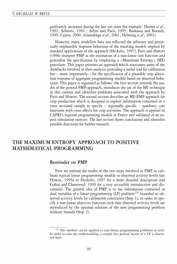
gnificantly increased during the last ten years (for example : Horner et al.,1992 ; Schmitz, 1994 ; Arfini and Paris, 1995; Barkaoui and Butault,1999 ; Cypris, 2000 ; Graindorge et al., 2001 ; Helming et al., 2001).

However, many modellers have not reflected the arbitrary and poten-tially implausible response behaviour of the resulting models implied bystandard applications of the approach (Heckelei, 1997). Paris and Howitt(1998) interpret PMP as the estimation of a non-linear cost function andgeneralize the specification by employing a «Maximum Entropy» (ME)procedure. This paper presents an approach which overcomes some of thedrawbacks involved in their analysis, providing a useful tool for calibrationbut – more importantly – for the specification of a plausible crop alloca-tion response of aggregate programming models based on observed beha-viour. This paper is organised as follows : the first section reminds the rea-der of the general PMP-approach, introduces the use of the ME techniquein this context and identifies problems associated with the approach byParis and Howitt. The second section describes an ME-PMP approach forcrop production which is designed to exploit information contained in across sectional sample to specify – regionally specific – quadratic costfunctions with cross effects for crop activities. The approach is applied toCAPRI’s regional programming models in France and validated in an ex-post simulation exercise. The last section draws conclusions and identifiespossible directions for further research.

THE MAXIMUM ENTROPY APPROACH TO POSITIVEMATHEMATICAL PROGRAMMING

Reminder on PMP

First we remind the reader of the two steps involved in PMP to cali-brate typical linear programming models to observed activity levels (seeHowitt, 1995a or Heckelei, 1997 for a more detailed description andGohin and Chantreuil, 1999 for a very accessible introduction and dis-cussion). The general idea of PMP is to use information contained indual variables of a linear programming (LP) problem (4) bounded to ob-served activity levels by calibration constraints (Step 1), in order to spe-cify a non-linear objective function such that observed activity levels arereproduced by the optimal solution of the new programming problemwithout bounds (Step 2).

(5) Matrices and vectors are printed in bold letters.(6) The calibration constraints are expressed as upper bounds on activity levels.

This is sufficient as long as the realisation of the activity provides a positive contri-bution to the objective function. This should be the case for expected profits if posi-tive activity levels are observed. When using realised yields and prices of a calibra-tion year, however, negative profits per activity may occur so that calibrationconstraints must be formulated as lower bounds as well.

POSITIVE MATHEMATICAL PROGRAMMING

31

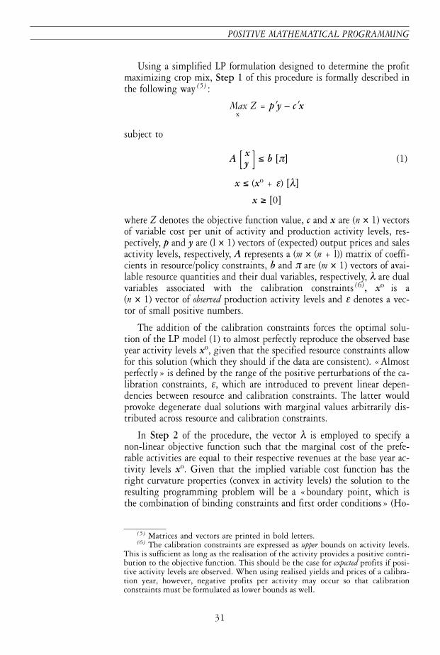
Using a simplified LP formulation designed to determine the profitmaximizing crop mix, Step 1 of this procedure is formally described inthe following way (5) :

Max Z = p′y – c′xx

subject to

xA [ ] ≤ b [π] (1)y

x ≤ (xo + ε) [λ]

x ≥ [0]

where Z denotes the objective function value, c and x are (n × 1) vectorsof variable cost per unit of activity and production activity levels, res-pectively, p and y are (l × 1) vectors of (expected) output prices and salesactivity levels, respectively, A represents a (m × (n + l)) matrix of coeffi-cients in resource/policy constraints, b and π are (m × 1) vectors of avai-lable resource quantities and their dual variables, respectively, λ are dualvariables associated with the calibration constraints (6), xo is a(n × 1) vector of observed production activity levels and ε denotes a vec-tor of small positive numbers.

The addition of the calibration constraints forces the optimal solu-tion of the LP model (1) to almost perfectly reproduce the observed baseyear activity levels xo, given that the specified resource constraints allowfor this solution (which they should if the data are consistent). «Almostperfectly» is defined by the range of the positive perturbations of the ca-libration constraints, ε, which are introduced to prevent linear depen-dencies between resource and calibration constraints. The latter wouldprovoke degenerate dual solutions with marginal values arbitrarily dis-tributed across resource and calibration constraints.

In Step 2 of the procedure, the vector λ is employed to specify anon-linear objective function such that the marginal cost of the prefe-rable activities are equal to their respective revenues at the base year ac-tivity levels xo. Given that the implied variable cost function has theright curvature properties (convex in activity levels) the solution to theresulting programming problem will be a «boundary point, which isthe combination of binding constraints and first order conditions» (Ho-

(7) Paris and Howitt (1998) show the general applicability of their approach alsowith respect to other functional forms. Compared to equation (2) they choose, howe-ver, a somewhat restricted quadratic functional form by excluding linear parameters.

(8) See Golan, Judge and Miller (1996) for a comprehensive introduction toMaximum Entropy Econometrics, or Mittelhammer, Judge, and Miller (2000),chapter E3, in the context of a general Econometrics textbook.


32

witt, 1995a, p. 330) and equal to the results of (1) with respect to acti-vity levels and dual values on the resource constraints, π.

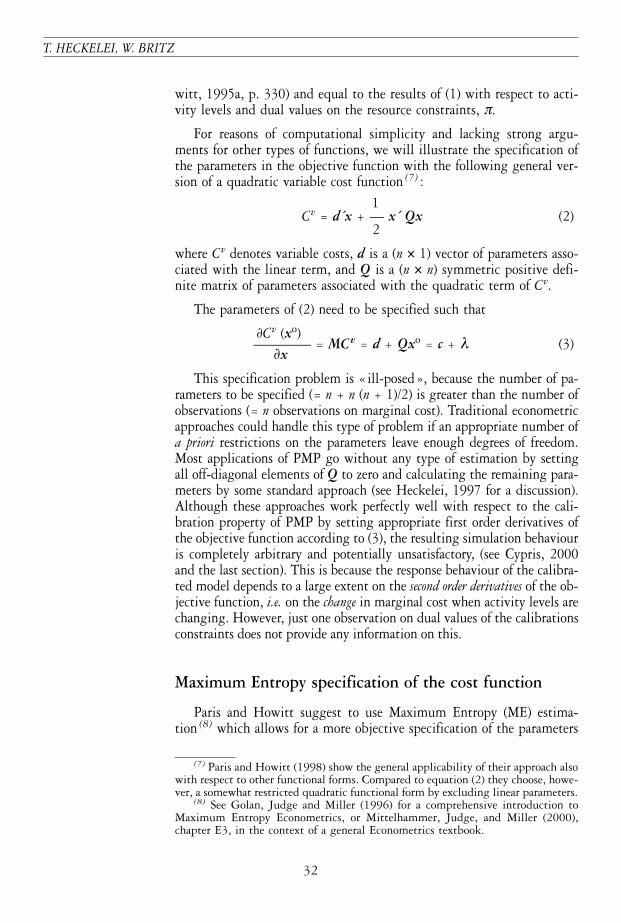
For reasons of computational simplicity and lacking strong argu-ments for other types of functions, we will illustrate the specification ofthe parameters in the objective function with the following general ver-sion of a quadratic variable cost function (7) :

1Cv = d´x + — x´ Qx (2)

2

where Cv denotes variable costs, d is a (n × 1) vector of parameters asso-ciated with the linear term, and Q is a (n × n) symmetric positive defi-nite matrix of parameters associated with the quadratic term of Cv.

The parameters of (2) need to be specified such that

∂Cv (xo)———— = MCv = d + Qxo = c + λ (3)

∂x

This specification problem is « ill-posed», because the number of pa-rameters to be specified (= n + n (n + 1)/2) is greater than the number ofobservations (= n observations on marginal cost). Traditional econometricapproaches could handle this type of problem if an appropriate number ofa priori restrictions on the parameters leave enough degrees of freedom.Most applications of PMP go without any type of estimation by settingall off-diagonal elements of Q to zero and calculating the remaining para-meters by some standard approach (see Heckelei, 1997 for a discussion).Although these approaches work perfectly well with respect to the cali-bration property of PMP by setting appropriate first order derivatives ofthe objective function according to (3), the resulting simulation behaviouris completely arbitrary and potentially unsatisfactory, (see Cypris, 2000and the last section). This is because the response behaviour of the calibra-ted model depends to a large extent on the second order derivatives of the ob-jective function, i.e. on the change in marginal cost when activity levels arechanging. However, just one observation on dual values of the calibrationsconstraints does not provide any information on this.

Maximum Entropy specification of the cost function

Paris and Howitt suggest to use Maximum Entropy (ME) estima-tion (8) which allows for a more objective specification of the parameters

(9) See Paris and Howitt (1998) for further details and a more extensive moti-vation of the approach.

(10) The variance of the maximum entropy estimates is negatively correlatedwith the number of support points defined and has a limit value for an infinitenumber of support points (see Golan et al., 1996, p. 139). There is no general rulefor the « right » number of support points, but tests with our models have shownthat choosing more than 4 support points does not change the numerical results ofthe calculated parameter expectations by an extent of any practical relevance.


33

of the non-linear cost function based on an « econometric type » crite-rion. Moreover, it has the potential of incorporating more than one ob-servation on activity levels into the specification of the parameters anddecreases the need to decide on exact a priori restrictions on the parame-ters. The application of ME to the calibration of programming modelscomes at a time of significantly increased general interest in entropytechniques by agricultural economists after the comprehensive introduc-tion by Golan et al. (1996). Their framework based on probability sup-ports of parameters and error terms allowed to apply the entropy crite-rion to ill-posed problems in econometrics. Studies in the realm ofproduction economics often focus on the estimation of input allocationto products and estimation of production technologies (for example :Lence and Miller, 1998a and 1998b ; Léon et al., 1999 ; Zhang and Fan,2001). Applications to dual behavioural models are, so far, less fre-quently observed (Oude Lansink, 1999). Note that this article should ra-ther be seen in the context of the PMP literature and consequently doesnot focus on contributions to the application of entropy techniques ingeneral. However, below we draw upon various of the already mentionedpublications when specifying the calibration approach.

To make ME-estimation of the variable cost function (2) operatio-nal (9), we first need to define support points for the parameter vector dand the matrix Q. One could centre the linear parameters d around theobserved accounting cost per unit of the activity, c. For example, wecould choose 4 support points for each parameter by setting (10)

– 2 . ci0 . cizdi = [ ] ∀i (4)+ 2 . ci

+ 4 . ci

In the case of the Q matrix we have to distinguish the diagonal(= change in marginal cost of activity i with respect to the level of activityi) from the off-diagonal elements (= change in marginal cost of activity iwith respect to the level of activity j). Given that the a priori expectationfor the linear parameter vector d are the accounting costs (supports cen-tred around ci in equation (4)), it is consistent with condition (3) to centrethe support points for qii around λi/x

oi and the off – diagonal elements qij

around zero. The centre of the support points λi/xoi for the diagonal ele-

ments are positive, a necessary condition for convexity of Cv.


34

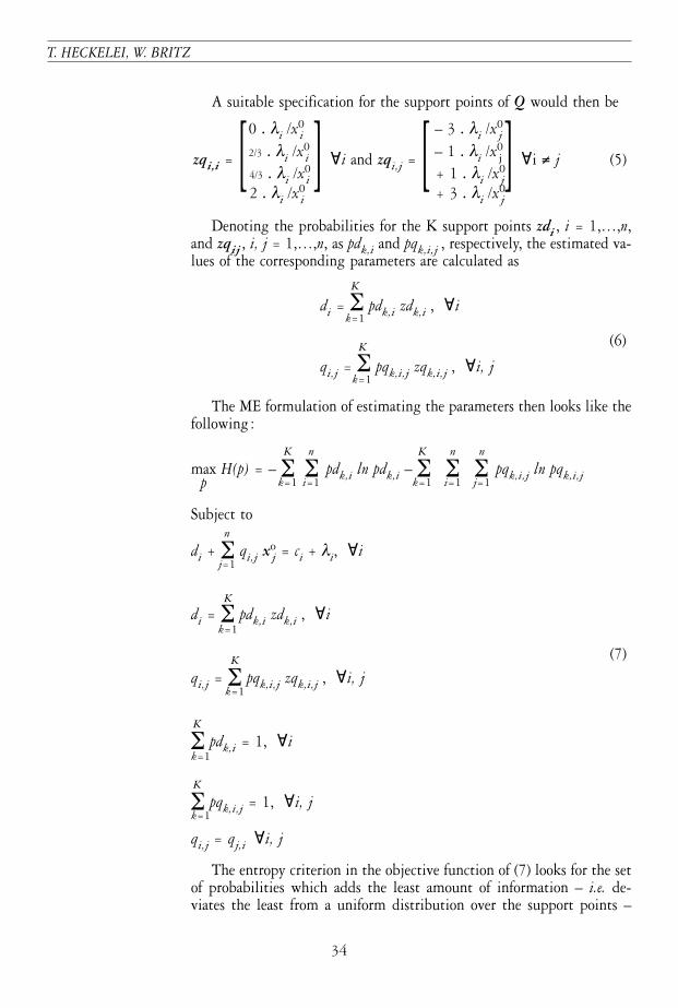
A suitable specification for the support points of Q would then be

0 . λi /x0i – 3 . λi /x0

j

2/3 . λi /x0i – 1 . λi /x0

jzqi,i = [ ] ∀i and zqi,j = [ ] ∀i ≠ j (5)4/3 . λi /x

0i + 1 . λi /x

0j

2 . λi /x0i + 3 . λi /x

0j

Denoting the probabilities for the K support points zdi , i = 1,…,n,and zqij , i, j = 1,…,n, as pdk,i and pqk,i,j , respectively, the estimated va-lues of the corresponding parameters are calculated as

K

di = Σ pdk,i zdk,i , ∀ik=1

K (6)

qi,j = Σ pqk,i,j zqk,i,j , ∀i, j k=1

The ME formulation of estimating the parameters then looks like thefollowing :

K n K n n

max H(p) = – Σ Σ pdk,i ln pdk,i – Σ Σ Σ pqk,i,j ln pqk,i,jp k=1 i=1 k=1 i=1 j=1

Subject ton

di + Σ qi,j xoj = ci + λi, ∀i

j=1

K


K (7)

qi,j = Σ pqk,i,j zqk,i,j , ∀i, jk=1

K

Σ pdk,i = 1, ∀ik=1

K

Σ pqk,i,j = 1, ∀i, jk=1

qi,j = qj,i ∀i, j

The entropy criterion in the objective function of (7) looks for the setof probabilities which adds the least amount of information – i.e. de-viates the least from a uniform distribution over the support points –

K


K (6)

qi,j = Σ pqk,i,j zqk,i,j , ∀i, j k=1

(11) Parameters can be easily defined for the diagonal elements of Q withoutthe need to apply a ME approach if just own-price elasticities are given, see forexample Helming et al. (2001).


35

but satisfies the explicitly shown « data constraint » of the estimationproblem being the marginal cost condition (3).

At this point we need to hold for a moment and need to address thequestion under what conditions a ME formulation for estimating the para-meters of the quadratic cost function deems useful. If we have only a(1 × n) vector of marginal cost available (from calibrating one linear pro-gramming problem to one base year solution), the outcome of the estima-tion and hence the simulation behaviour of the resulting model will beheavily dominated by the supports. Such an application of ME shouldhence be interpreted as calibrating a cost function based on prior expecta-tions on the parameter values to observed values according to condition(3). The entropy criterion works here as a penalty function for the devia-tion from the prior expectations (centre of supports) and the term «estima-tion for the calibration process» may be misleading. The approach with justone observation on marginal cost could be sensibly applied to derive a costfunction based on specific prior information, for example a full matrix ofelasticities (11) or to exogenously given yield functions (Howitt, 1995a).

The example defined according to (4) and (5) is however not a mea-ningful application for such a calibration process as supports were definedwithout any valuable prior information on the cost function. Specifically,the ME problem will reach its optimum when the probabilities follow auniform distribution, since the centres of the support values already sa-tisfy the data constraints. The resulting parameter estimates will beexactly the ones implied by the « standard approach» as defined in Hec-kelei (1997), i.e. linear parameters of the cost function are equal to therespective activity’s accounting costs ci, the off-diagonal elements of theQ matrix are zero, and the diagonal elements are equal to λi/x

oi. The si-

mulation behaviour of the resulting model is arbitrary as it completelydepends on the arbitrary specification of the support values.

For similar reasons, the approach of Paris and Howitt (1998) who repa-rameterize the Q matrix based on a LDL′ (Cholesky) decomposition to en-sure appropriate curvature properties of the estimated cost function should– in our view – only be seen as a demonstration on how to combine MEand PMP. The choice of their support values is not based on prior informa-tion. They centre the elements of D around the value for the diagonal ele-ments of Q which would satisfy the marginal cost condition and the ele-ments of L around zero. Due to the complex (and even order-dependent)relationship between the matrices L, D and Q, this implies rather non-transparent a priori expectations for the parameters of Q. The nonzero crosscosts effects of activities obtained from their ME solution is merely basedon this technically motivated choice of support points.


36

In contrast to the examples given above, we now suggest an approachbased on a cross-sectional sample of marginal cost from a set of regional pro-gramming models. We apply the term «estimation» for this procedure,since several regional vectors of marginal costs are used to specify the costfunctions. The choice of ME instead of other estimators is motivated by thefact that we have still negative degrees of freedom. The discussion willmostly concentrate on necessary parametric restrictions across regions to ac-commodate for regions with different sizes and crop rotations. Additionally,we provide a solution to the curvature problem which allows the definitionof support points for the actual parameters to be estimated by incorporatinga LL′ decomposition as direct constraints of the estimation problem.

A PMP-ME APPROACH BASED ON A CROSSSECTIONAL SAMPLE

The first part of this section presents a rationale for the approach andintroduces the most important parts of the mathematical formulation.The second part delivers some details on an application for CAPRI’s re-gional programming models for France and presents results of an ex-postvalidation for the simulation behaviour of the specified model across theCAP-reform of 1992.

RationaleOur objective here is to estimate a quadratic cost function with cross

cost effects (full Q matrix) between crop production activities. Suppose onecan generate R (1 × n) vectors of marginal costs from a set of R regionalprogramming models by applying the first step of PMP. In our example,n represents 18 crops and R the 22 French NUTS-2 regions. In order toexploit this information for the specification of quadratic cost functionsfor all regions, we need to define appropriate restrictions on the parame-ters across regions, since otherwise no informational gain is achieved.

Consider the following suggestion for a regional vector of marginalcost :

MCvr = dr + Qr xr (8)

Qr = (cpir)g Sr BS′r with

where dr is a (n × 1) vector of linear cost function parameters in regionr, Qr represents a (n × n) matrix of quadratic cost term parameters in re-gion r, cpir stands for regional « crop profitability index» defined as therelation between the regional and average revenue per hectare(p′yr /Lr)/(Σp′yr /ΣLr) where Lr is land available, g is a parameter deter-

r r

oir

iir xs

,,,

1=


37

mining the influence of the crop profitability index, Sr constitutes(n × n) diagonal scaling matrices for each region r, and finally B is a(n × n) parameter matrix related to Qr.

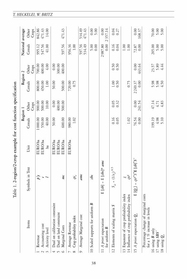
The rationale for (8) can best be inferred from a didactic exampleshown in table 1, based on a LP model with 2 crops, 2 regions and aland constraint. Rows 1-3 present the observed base year data – total re-venues, accounting costs and activity levels – from which the duals ofthe calibration constraints, marginal costs (rows 4-6) as well as averagerevenues and the crop profitability index (row 7-8) can be deducted.

Contrary to the ultimate application, the matrix B as shown in thelast columns of row 11 is given and not estimated. It is defined suchthat the relative increase of marginal costs for a 1 % increase in levels isequal to 5 % at national level. In order to motivate the scaling with Sr ,we have a look at the implied elasticities of marginal costs to changes inactivity levels as shown in row 16 if the scaling vectors S are left out. Inthat case, elasticities are a direct function of observed activity levels : thesmaller the level, the smaller the elasticity. Including the scaling vectors,as shown in row 17, provides a more plausible parameter restriction.

The term (cpir)g which reflects differences in regional profitability is sup-

posed to capture the economic effect of differences in soil, climaticconditions etc. The magnitude of the effect on the marginal cost func-tion estimated by the exponent g. A negative g, for example, wouldimply that specialising in a certain crop is penalised less in a region withcropping conditions above average since, ceteris paribus, Qr is smallerthan average in this case.

The overall specification implies that – apart from the effect of thecrop profitability index – the Qr’s are identical for regions with the samecrop rotation. We motivated the use of more than one observation by thefact that second order derivatives of the cost function strongly influencethe simulation behaviour of the model. Where does this informationhide in equation (8) ? Observed rotations and marginal costs recoveredby the calibration step differ between regions. The matrix B – commonacross regions – is estimated as to describe the differences in marginalcosts depending on the differences in levels. The parameters are now es-timated such that changing region i’s rotation to the rotation in regionj causes changes in marginal cost matching the observed differences bet-ween the two regions (again apart from the effect of the crop profitabi-lity index). This is the important contribution of the cross-sectional ana-lysis : the simulation behaviour resulting from the ME problems is notlonger depending in an arbitrary way on the support points, but is basedon a clear hypothesis about the relation between crop rotation and mar-ginal costs.


38

Tabl

e 1.

2-re

gion

/2-c

rop

exam

ple

for

cost

fun

ctio

n sp

ecifi

catio

n

Reg

ion

1R

egio

n 2

Nat

iona

l ave

rage

Item

sSy

mbo

ls in

Tex

tU

nit

Cer

eals

Oth

er

Cer

eals

Oth

er

Cer

eals

Oth

er

Cro

psC

rops

Cro

ps1

Rev

enue

p′y

EUR

O/h

a1

000.

0090

0.00

800.

0070

0.00

995.

1284

2.86

2A

ccou

ntin

g co

stc

EUR

O/h

a55

0.00

500.

0045

0.00

400.

0054

7.56

471.

433

Act

ivit

y le

vel

lha

40.0

010

.00

1.00

4.00

41.0

014

.00

4D

ual o

n ca

libra

tion

con

stra

int

EUR

O/h

a50

.00

0.00

50.0

00.

005

Dua

l on

land

con

stra

int

EUR

O/h

a40

0.00

300.

006

Mar

gina

l Cos

tsm

cEU

RO

/ha

600.

0050

0.00

500.

0040

0.00

597.

5647

1.43

7A

vera

ge R

even

ueEU

RO

/ha

980.

0072

0.00

956.

368

Cro

p pr

ofita

bilit

y in

dex

cpir

1.02

0.75

1.00

9A

vera

ge M

argi

nal c

ost

amc

597.

5653

4.49

534.

4947

1.43

10Sc

aled

sup

port

s fo

r un

iform

Bzb

s5.

000.

000.

005.

00

11A

pri

ori e

xpec

tati

on

E [z

b]=

E [z

bs]*

am

c2

987.

800.

00fo

r un

iform

B0.

002

357.

14

12El

emen

ts o

f sca

ling

mat

rix

SS ii

=(1

/xi)

0.5

0.16

0.05

1.00

0.50

0.16

0.04

0.05

0.32

0.50

0.50

0.04

0.27

13Ex

pone

nt o

f cro

p pr

ofit

abili

ty in

dex

g1.

0014

Influ

ence

of c

rop

prof

itab

ility

inde

xcp

ig1.

020.

751.

00

15A

pri

orie

xpec

tati

on Q

rE

[Qr]

=cp

ig*S* E

[zb]

* S′76

.54

0.00

224

9.37

0.00

72.8

70.

000.

0024

1.54

0.00

443.

640.

0016

8.37

Perc

enta

ge c

hang

e of

mar

gina

l cos

ts

for

a 1

% in

crea

se in

leve

ls16

usin

g B

only

199.

1947

.14

5.98

23.5

720

5.00

70.0

017

usin

g SB

S ′4.

984.

715.

985.

895.

005.

0018

usin

g Q

r5.

104.

834.

504.

445.

005.

00

(12) The two different forms of the Cholesky decompositions are related in thefollowing way : Replacing the « ones » on the diagonal triangular matrix L of Q= LDL′ with the square roots of the corresponding diagonal elements of D allowsto write Q = LL′.


39

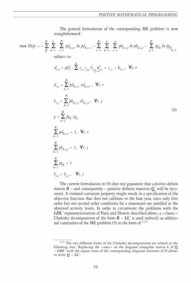
The general formulation of the corresponding ME problem is nowstraightforward :

K n R K n n K

max H(p) = – Σ Σ Σ pdk,i,r ln pdk,i, r – Σ Σ Σ pbk,i,j ln pbk,i,j – Σ pgk ln pgkp k=1 i=1 r=1 k=1 i=1 j=1 k=1

subject ton

di,r + cpigr . Σ si,i sj,j bi,j xo

j,r = ci,r + λi,r , ∀i, rj=1

K

di,r = Σ pdk,i,r zdk,i,r , ∀i, rk=1

K

bi,j = Σ pbk,i,j zbk,i,j , ∀i, jk=1

K (9)g = Σ pgk zgk

k=1

K

Σ pdk,i,r = 1, ∀i, rk=1

K

Σ pbk,i,j = 1, ∀i, jk=1

K

Σ pgk = 1k=1

bi,j = bj,i , ∀i, j

The current formulation in (9) does not guarantee that a positive definitematrix B – and consequently – positive definite matrices Qr will be reco-vered. A violated curvature property might result in a specification of theobjective function that does not calibrate to the base year, since only firstorder but not second order conditions for a maximum are satisfied at theobserved activity levels. In order to circumvent the problems with theLDL′ reparameterisation of Paris and Howitt described above, a «classic»Cholesky decomposition of the form B = LL′ is used indirectly as additio-nal constraints of the ME problem (9) in the form of (12)

(13) In earlier tests, a pragmatic solution was chosen for the curvature problemby forcing the first and second order minors of B to have the appropriate sign andrestricting all off-diagonal elements to be smaller than diagonal elements duringthe ME step. The resulting matrix was then – if necessary – treated by a so-called« modified» Cholesky-decomposition which ensures definiteness by employing op-timal correction factors to the diagonal elements (Gill et al., 1989, p. 108). Thisprocedure has proven to be operational for very large matrices.


40

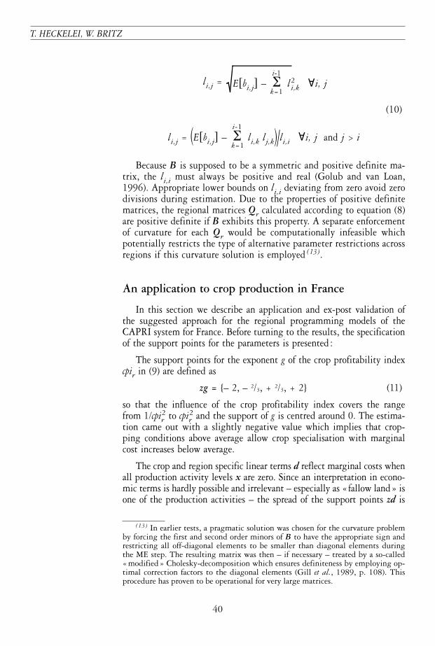
li,j =(

(10)

i-1

li,j = (E[bi,j] – Σ li,k lj,k)"li,i ∀i, j and j > ik=1

Because B is supposed to be a symmetric and positive definite ma-trix, the li,i must always be positive and real (Golub and van Loan,1996). Appropriate lower bounds on li,i deviating from zero avoid zerodivisions during estimation. Due to the properties of positive definitematrices, the regional matrices Qr calculated according to equation (8)are positive definite if B exhibits this property. A separate enforcementof curvature for each Qr would be computationally infeasible whichpotentially restricts the type of alternative parameter restrictions acrossregions if this curvature solution is employed (13).

An application to crop production in France

In this section we describe an application and ex-post validation ofthe suggested approach for the regional programming models of theCAPRI system for France. Before turning to the results, the specificationof the support points for the parameters is presented :

The support points for the exponent g of the crop profitability indexcpir in (9) are defined as

zg = {– 2, – 2/3, + 2/3, + 2} (11)

so that the influence of the crop profitability index covers the rangefrom 1/cpir

2 to cpir2 and the support of g is centred around 0. The estima-

tion came out with a slightly negative value which implies that crop-ping conditions above average allow crop specialisation with marginalcost increases below average.

The crop and region specific linear terms d reflect marginal costs whenall production activity levels x are zero. Since an interpretation in econo-mic terms is hardly possible and irrelevant – especially as « fallow land» isone of the production activities – the spread of the support points zd is

[ ] lbE1i

1k

2k,ii,i −�

−

=

i-1E[bi,j] – Σ l2

i,k ∀i, jk=1

(14) With this support point formulation, the linear terms dr can actually beviewed as the sum of a predetermined parameter vector cr and a crop and regionspecific error term which is centred around zero. Consequently, the specification isnumerically equivalent to a generalised ME formulation with error terms. Weopted for the representation above, because the « error term » is ultimately kept inthe specification of the objective function so that the resulting programming mo-dels calibrate exactly to observed activity levels.

(15) See also Golan et al. for a discussion of « Normalised Entropy » and its usein various applications.

(16) Generally, prior expectations are defined as a weighted average of support va-lues. In the ME case, the weights are probabilities following a uniform distribution. Inthe CE case, the weights are the probabilities as defined by the reference distribution.


41

consequently set to a very wide interval around the observed costs. Thespread is 180 times the national average in revenue per ha (14).

zd = cr + {– 90, – 30, 30, 90} Σ p′yr / Σ Lr (12)r r

Let —MCi

—be the land-weighted average of marginal cost for crop i

across regions. The support points for B are then defined as follows (seerows 9-11 in Table 1 as well) :

zbi,j = zbsi,j amci,jwhere

{0.001, 3.3, 6.66, 10} ∀i = j (13)zbsi,j = [ {– 2, – 2/3, 2/3, 2} ∀i ≠ j ] and

amci,j = 1/2 ( —MCi

—+

—MCj

—)

According to the spread defined by zbs, the supports zb for B are defi-ned such that changing the activity level of crop i by 1 % increases owncosts between zero and ten percent. The cross effects are symmetrically cen-tred around zero and allow for a change between – 2 % and +2 % of theaverage marginal costs of crop i and j, amc. This support point definitionclearly introduces prior information. The elements of B will be drawn to-wards the centre of the support intervals by the entropy criterion as muchas the data constraints allow. In addition we excluded (the theoretically im-possible) negative values for the diagonal elements and restricted the crosseffects to be small relative to the own activity level effects on marginalcost. Nevertheless, the spread of the support points specification leavesconsiderable freedom for obtaining a wide range of implied elasticities.

The determination of support points in the context of ME and GME(Generalised ME which includes error terms in data constraints) is a de-licate problem and therefore deserves some further discussion : thereseems to be a great desire to determine support points objectively and toavoid prior information as much as possible. Léon et al. (1999), forexample, employ the normalised entropy measure to judge the «superio-rity» of different (predefined) symmetric and asymmetric support pointspecifications (15). This measure reaches its maximum when the estimatedparameters do not deviate at all from the a priori expectations defined bythe support values (16). Consequently, it allows to compare different sup-


42

port point specifications with respect to their compatibility with the dataconstraints. The measure does not allow, however, to identify an optimalset of support values for an underdetermined estimation problem. Just asthere is an infinite number of parameter vectors satisfying the dataconstraints, there is as well an infinite number of support definitionswith prior expectation equal to these parameter vectors. All these supportpoint specifications obtain the same value of the normalised entropy mea-sure, but not the same parameter estimates. Therefore, we did not consi-der this measure for the choice of support values here.

Other researches focussing on the idea of using purely «data-based»supports (van Akkeren et al., 2001) show advantages over classical esti-mation techniques in some ill-conditioned (e.g. multicollinear) data si-tuations but well posed with respect to the number of observations.Those techniques obviously cannot make up for limited data informa-tion. From our point of view it should simply be accepted that a smallnumber of observations relative to the number of parameters imply littleinformation and that ME and GME succeed in these situations, only be-cause they allow to flexibly incorporate prior information by restrictingthe parameter space. There is certainly the danger of introducing astrong bias if the prior is formulated very tight and far off the truevalue. In the GME context, however, it can be taken as some comfortthat the estimator is consistent under general regularity conditions aslong as the true value of the parameters is within the support range (seeMittelhammer and Cardell, 2000).

Above, we tried to make our a priori information as transparent aspossible and chose to use a uniform distribution where the centres arethe prior expectations. Note that this is numerically equivalent to across entropy (CE) approach with this uniform distribution serving asthe reference distribution. Other possibilities to represent prior informa-tion include differentiated prior weights in the CE reference distributionor asymmetric support point spacing in ME and CE contexts. These me-thods provide flexibility in expressing just the prior information that isavailable, but – to our knowledge – there is no objective criterion thatmakes one approach generally superior to the others. At some point,there might be measures to compare the penalty involved for deviatingfrom the prior information for the different approaches and this will im-prove transparency (see Preckel, 2001 for looking at the entropy crite-rion from a penalty view).

Returning from this general support point discussion to our specificcase, we repeat that the specifications in (12) and (13) imply some priorinformation, but the support spread leaves considerable ranges for theparameters. Also the influence of the support points on the estimationoutcomes becomes considerably smaller with an increasing number ofobservations and allowing for this to happen is a major objective of ourapproach in contrast to previous PMP applications.


43

The approach discussed in the previous section estimates a non-linearcost function depending on crop production activity levels based on ob-served regional differences in marginal costs at just one point in time.Naturally, doubt may be raised if that cross-sectional information can bejust mapped in the time domain by assuming that changes in crop rota-tion over time in each single region have a similar effect on variablecosts as the differences in observed crop rotations for a set of regions atone point of time. We consequently check the resulting simulation be-haviour of the models in an ex-post simulation exercise.

We took three year averages both for the calibration and simulationyear based on data in the CAPRI data base for the 22 NUTS-2 regionsin France. Given data availability, we used years 1989 to 1991 («1990»)for the calibration and 1993 to 1995 («1994») for the simulation. Themove from 1991 to 1994 has the advantage that the 1992 CAP-reformlays just in between which offers a good opportunity to test the modelunder a significant policy change. However, some restrictions apply : Wehad no data on the participation in voluntary set-aside programs beforethe CAP-reform – therefore important information was left out in thecalibration step. Naturally, no data on obligatory set-aside and non-foodproduction, both introduced by the 1992 CAP-reform, entered the cali-bration for 1990. We therefore had to make some assumptions regardingthese activities :

• The parameters in d and B relating to voluntary and obligatory setaside were set equal to the ones obtained for fallow land in 1990, assu-ming that they have the same rotational effects as represented by thecost function. Nevertheless, voluntary and obligatory set-aside are stilltreated in simulation according to the policy formulation in the CAP-re-form, i.e. they are linked to the production of «grandes cultures » in theappropriate way (see below).

• The driving forces of non-food production on set-aside were unknownto us with respect to hard quantitative information. Therefore, we fixednon-food production to known levels in 1994. As non-food has a sharearound 10 % on oilseeds in total, the resulting improvement in themodel’s fit is not dramatic. We also applied this assumption to the otherapproaches which are compared to our ME-PMP calibrated model.

The set-aside regulation is modelled by constraints : the obligationmust be fulfilled by an appropriate level of obligatory set-aside or non-food production on set-aside. Voluntary set-aside may be added as longas the sum of total set-aside including non-food production does not ex-ceed 33 % of the endogenously determined «grandes cultures » area. Pre-mia are cut if regional base areas are exceeded. As the presented ME-PMP approach is only suitable for annual crops, we fixed animalproduction and perennials to observed levels in 1994. Apart from thesugar beet quota and the land restriction, no other constraints enter themodel specification.


44

The ME problem (9) was successfully solved with the General Alge-braic Modelling System (GAMS) using the solver CONOPT2. It shouldbe noted here that a powerful solver for this type of optimisation pro-blem is necessary, especially due to the considerable non-linearity intro-duced by the Cholesky decomposition constraints (10).

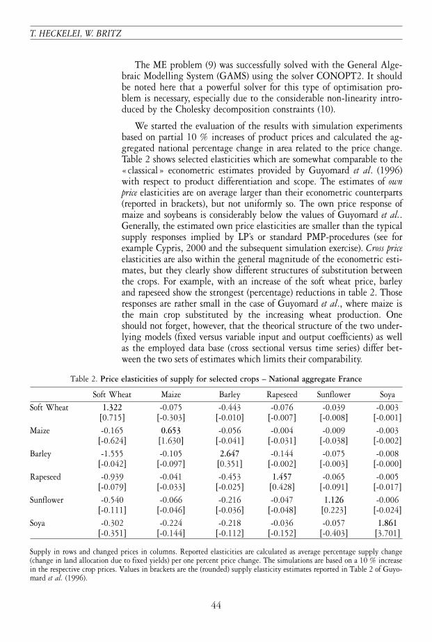
We started the evaluation of the results with simulation experimentsbased on partial 10 % increases of product prices and calculated the ag-gregated national percentage change in area related to the price change.Table 2 shows selected elasticities which are somewhat comparable to the«classical» econometric estimates provided by Guyomard et al. (1996)with respect to product differentiation and scope. The estimates of ownprice elasticities are on average larger than their econometric counterparts(reported in brackets), but not uniformly so. The own price response ofmaize and soybeans is considerably below the values of Guyomard et al..Generally, the estimated own price elasticities are smaller than the typicalsupply responses implied by LP’s or standard PMP-procedures (see forexample Cypris, 2000 and the subsequent simulation exercise). Cross priceelasticities are also within the general magnitude of the econometric esti-mates, but they clearly show different structures of substitution betweenthe crops. For example, with an increase of the soft wheat price, barleyand rapeseed show the strongest (percentage) reductions in table 2. Thoseresponses are rather small in the case of Guyomard et al., where maize isthe main crop substituted by the increasing wheat production. Oneshould not forget, however, that the theorical structure of the two under-lying models (fixed versus variable input and output coefficients) as wellas the employed data base (cross sectional versus time series) differ bet-ween the two sets of estimates which limits their comparability.

Table 2. Price elasticities of supply for selected crops – National aggregate France

Soft Wheat Maize Barley Rapeseed Sunflower SoyaSoft Wheat 1.322 -0.075 -0.443 -0.076 -0.039 -0.003

[0.715] [-0.303] [-0.010] [-0.007] [-0.008] [-0.001]Maize -0.165 0.653 -0.056 -0.004 -0.009 -0.003

[-0.624] [1.630] [-0.041] [-0.031] [-0.038] [-0.002]Barley -1.555 -0.105 2.647 -0.144 -0.075 -0.008

[-0.042] [-0.097] [0.351] [-0.002] [-0.003] [-0.000]Rapeseed -0.939 -0.041 -0.453 1.457 -0.065 -0.005

[-0.079] [-0.033] [-0.025] [0.428] [-0.091] [-0.017]Sunflower -0.540 -0.066 -0.216 -0.047 1.126 -0.006

[-0.111] [-0.046] [-0.036] [-0.048] [0.223] [-0.024]Soya -0.302 -0.224 -0.218 -0.036 -0.057 1.861

[-0.351] [-0.144] [-0.112] [-0.152] [-0.403] [3.701]

Supply in rows and changed prices in columns. Reported elasticities are calculated as average percentage supply change(change in land allocation due to fixed yields) per one percent price change. The simulations are based on a 10 % increasein the respective crop prices. Values in brackets are the (rounded) supply elasticity estimates reported in Table 2 of Guyo-mard et al. (1996).


45

The comparison of the resulting partial supply responses with valuesof estimated behavioural functions is certainly interesting. However, theassessment of the simulation behaviour across larger economic and policychanges is closer to the ultimate purpose of our model. Therefore, we de-signed an ex-post simulation experiment as described above, results ofwhich are rarely generated in the context of programming models, butare very informative from our point of view.

In order to judge if the new methodology has comparative advan-tages, we included a « standard PMP» approach in the ex-post valida-tion as well. Here, only diagonal elements of B are specified such thatthe linear and quadratic terms for each production activity i implicitlydefine average variable cost matching the observed accounting cost ci forthe base year. In the case of the quadratic cost function this implies that

2λibi,i = —— and di = ci – λi ∀ i = 1, ..., n (14)x0

i

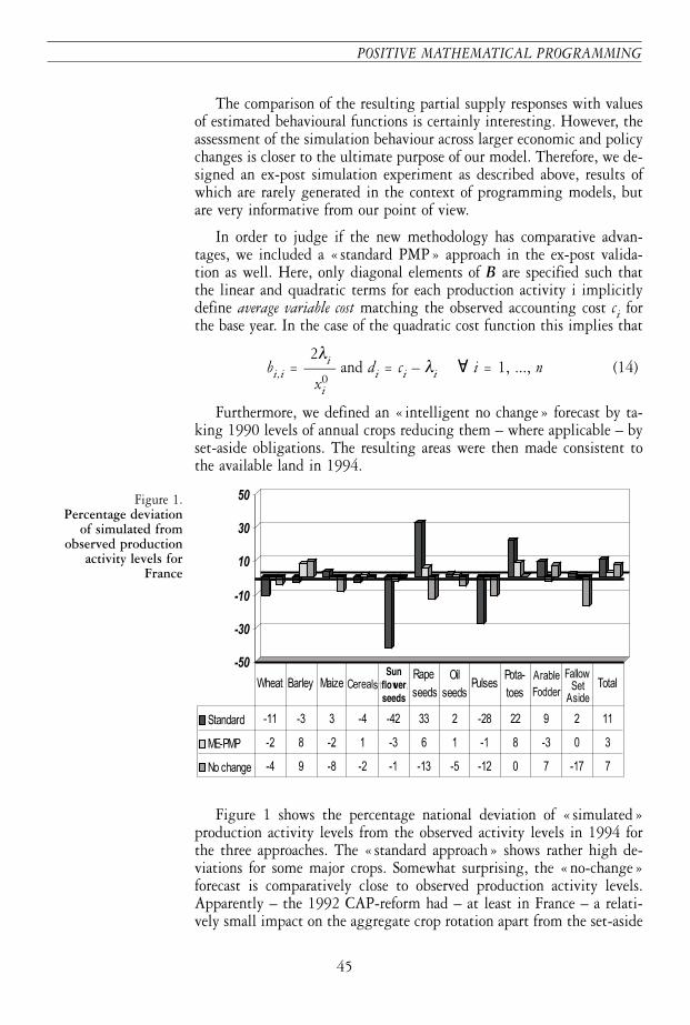
Furthermore, we defined an « intelligent no change » forecast by ta-king 1990 levels of annual crops reducing them – where applicable – byset-aside obligations. The resulting areas were then made consistent tothe available land in 1994.

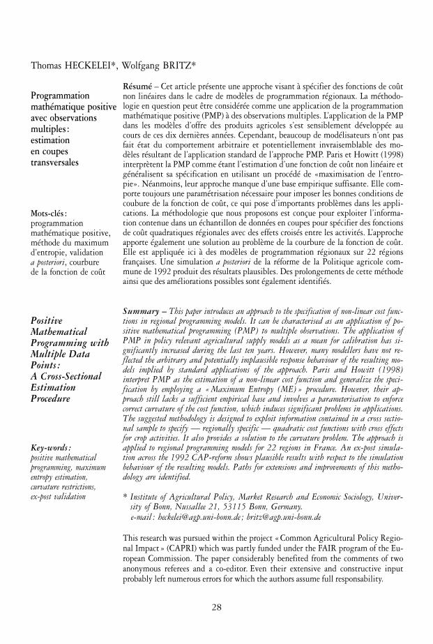
Figure 1 shows the percentage national deviation of « simulated»production activity levels from the observed activity levels in 1994 forthe three approaches. The « standard approach» shows rather high de-viations for some major crops. Somewhat surprising, the «no-change»forecast is comparatively close to observed production activity levels.Apparently – the 1992 CAP-reform had – at least in France – a relati-vely small impact on the aggregate crop rotation apart from the set-aside

Figure 1.Percentage deviation

of simulated fromobserved production

activity levels forFrance

Sunflowerseeds


46

effect. With this in mind, the fit of the ME-PMP approach based on thecross sectional sample is rather promising : apart from sunflowers andpotatoes it provides better simulated values than the «no-change» re-sults. The sum of absolute deviation in levels weighted by the observedlevels amounts just up to 3 % (see «Total»).

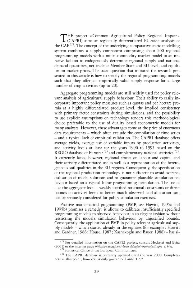
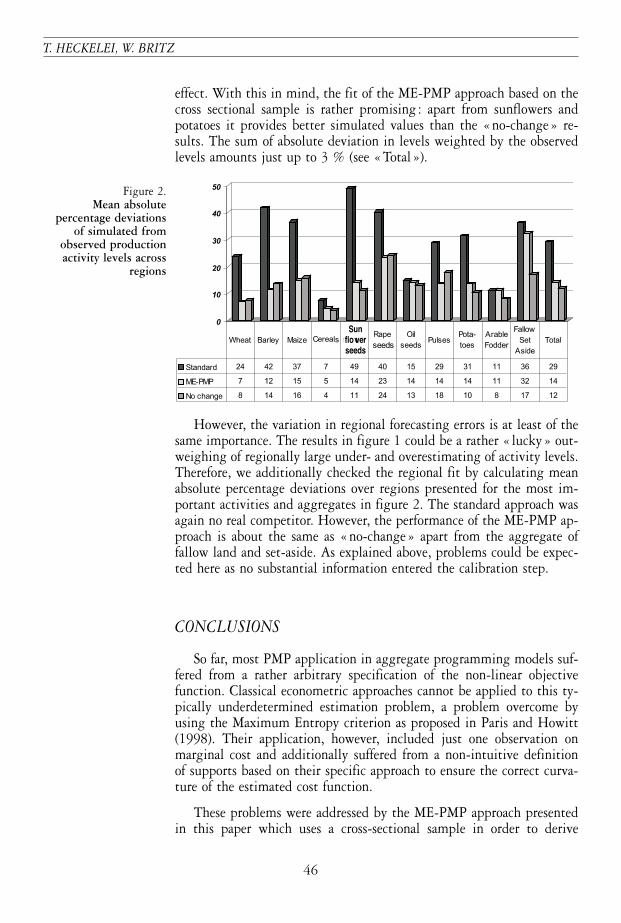
However, the variation in regional forecasting errors is at least of thesame importance. The results in figure 1 could be a rather « lucky » out-weighing of regionally large under- and overestimating of activity levels.Therefore, we additionally checked the regional fit by calculating meanabsolute percentage deviations over regions presented for the most im-portant activities and aggregates in figure 2. The standard approach wasagain no real competitor. However, the performance of the ME-PMP ap-proach is about the same as «no-change» apart from the aggregate offallow land and set-aside. As explained above, problems could be expec-ted here as no substantial information entered the calibration step.

CONCLUSIONS

So far, most PMP application in aggregate programming models suf-fered from a rather arbitrary specification of the non-linear objectivefunction. Classical econometric approaches cannot be applied to this ty-pically underdetermined estimation problem, a problem overcome byusing the Maximum Entropy criterion as proposed in Paris and Howitt(1998). Their application, however, included just one observation onmarginal cost and additionally suffered from a non-intuitive definitionof supports based on their specific approach to ensure the correct curva-ture of the estimated cost function.

These problems were addressed by the ME-PMP approach presentedin this paper which uses a cross-sectional sample in order to derive

Figure 2.Mean absolute

percentage deviationsof simulated from

observed productionactivity levels across

regions

Sunflowerseeds


47

changes in marginal cost based on observed differences between regionswith different crop rotations and provides a solution for the curvatureproblem with limited computational burden and direct definition ofsupport points for the parameters of interest.

An ex-post validation of the resulting model specification simulatedthe 1992 CAP-reform for crop production in France. The results show apromising fit of observed production activity levels – not only for thenational aggregate, but as well in the regional dimension. The ex-postsimulation exercise – rarely executed or published in the context of ag-gregate programming models – shows the validity of the calibrationprocedure for regional programming models. The allocation behaviour ofthe resulting models is clearly superior to a standard application of PMP.

Nevertheless, the general approach leaves ample opportunities forfurther research : Specific issues on our research agenda are the additio-nal use of time series observations to extend the information base and toestimate time dependant parameters, the introduction of estimated para-meters to describe the relationship between crop rotation and changes inmarginal cost and, last but not least, an explicit elaboration on the linksbetween PMP and duality based econometric models with explicit allo-cation of land to different production activities. The last issue could po-tentially improve the theoretical understanding of PMP which origina-ted as a rather pragmatic solution to calibration problems withagricultural programming models.

REFERENCES

ARFINI (F.), PARIS (Q.), 1995 — A positive mathematical program-ming model for regional analysis of agricultural policies, in :SOTTE (E.) (ed.), The Regional Dimension in Agricultural Economicsand Policies, EAAE, Proceedings of the 40th Seminar, June 26-28,Ancona, pp. 17-35.

BARKAOUI (A.), BUTAULT (J.-P.), 1999 — Positive mathematical pro-gramming and cereals and oilseeds supply within EU underAgenda 2000, Paper presented at the 9th European Congress ofAgricultural Economists, Warsaw, August.

CYPRIS (Ch.), 2000 — Positiv Mathematische Programmierung (PMP)im Agrarsektormodell RAUMIS, Dissertation, University ofBonn.


48

GILL (P. E.), MURRAY (W.) and WRIGHT (M. H.), 1989 — PracticalOptimisation, London, Academic Press.

GOHIN (A.), CHANTREUIL (F.), 1999 — La programmation mathéma-tique positive dans les modèles d’exploitation agricole. Principeset importance du calibrage, Cahiers d’économie et sociologie rurales,52, pp. 59-78.

GOLAN (A.), JUDGE (G.) and MILLER (D.), 1996 — Maximum EntropyEconometrics, Chichester, Wiley.

GOLUB (G. H.), VAN LOAN (C. F.), 1996 — Matrix Computations, 3rdedition, Baltimore, John Hopkins University Press.

GRAINDORGE (C.), DE FRAHAN (B.-H.) and HOWITT (R. E.), 2001— Analysing the effects of Agenda 2000 using a CES calibratedmodel of Belgian agriculture, in : HECKELEI (T.), WITZKE (H. P.)and HENRICHSMEYER (W.) (eds), 2000, Agricultural Sector Model-ling and Policy Information Systems, Proceedings of the 65th EAAESeminar, March 29-31, 2000, Kiel, Wissenschaftsverlag Vauk,pp. 177-186.

GUYOMARD (H.), BAUDRY (M.) and CARPENTIER (A.), 1996 — Esti-mating crop supply response in the presence of farm programmes :application to the CAP, European Review of Agricultural Economics, 23,pp. 401-420.

HECKELEI (T.), 1997 — Positive mathematical programming : Reviewof the standard approach, CAPRI-working paper 97-03, Univer-sity of Bonn.

HECKELEI (T.), BRITZ (W.), 2001 — Concept and explorative applica-tion of an EU-wide regional agricultural sector model (CAPRI-Projekt), in : HECKELEI (T.), WITZKE (H. P.), and HENRICHS-MEYER (W.) (eds), Agricultural Sector Modelling and PolicyInformation Systems, Proceedings of the 65th EAAE Seminar, March29-31, 2000, Kiel, Wissenschaftsverlag Vauk, pp. 281-290.

HELMING (J. F. M.), PEETERS (L.) and VEENDENDAAL (P. J. J.), 2001— Assessing the consequences of environmental policy scenariosin Flemish agriculture, in : HECKELEI (T.), WITZKE (H. P.), andHENRICHSMEYER (W.) (eds), Agricultural Sector Modelling and Po-licy Information Systems, Proceedings of the 65th EAAE Seminar,March 29-31, 2000, Kiel, Wissenschaftsverlag Vauk, pp. 237-245.

HORNER (G. L.), CORMAN (J.), HOWITT (R. E.), CARTER (C. A.) andMACGREGOR (R. J.), 1992 — The Canadian regional agriculturemodel : Structure, operation and development, Agriculture Ca-nada, Technical Report 1/92, Ottawa.


49

HOUSE (R. M.), 1987 — USMP regional agricultural model, Washing-ton DC, USDA, National Economics Division Report, ERS, 30.

HOWITT (R. E.), 1995a — Positive mathematical programming, Ame-rican Journal of Agricultural Economics, 77 (2), pp. 329-342.

HOWITT (R. E.), 1995b — A calibration method for agricultural eco-nomic production models, Journal of Agricultural Economics, 46,pp. 147-159.

HOWITT (R. E.), GARDNER (D. B.), 1986 — Cropping productionand resource interrelationships among California crops in responseto the 1985 food security act, in : Impacts of Farm Policy and Tech-nical Change on US and Californian Agriculture, Davis, pp. 271-290.

KASNAKOGLU (H.), BAUER (S.), 1988 — Concept and application ofan agricultural sector model for policy analysis in Turkey, in :BAUER (S.), HENRICHSMEYER (W.) (eds), Agricultural Sector Mo-delling, Kiel, Wissenschaftsverlag Vauk.

LENCE (H. L.), MILLER (D.), 1998a — Estimation of multioutput pro-duction functions with incomplete data : A generalized maximumentropy approach, European Review of Agricultural Economics, 25,pp. 188-209.

LENCE (H. L.), MILLER (D.), 1998b — Recovering output specific in-puts from aggregate input data : A generalized cross-entropy ap-proach, American Journal of Agricultural Economics, 80 (4), pp. 852-867.

LÉON (Y.), PEETERS (L.), QUINQU (M.) and SURRY (Y.), 1999 — Theuse of maximum entropy to estimate input-output coefficientsfrom regional farm accounting data, Journal of Agricultural Econo-mics, 50, pp. 425-439.

MITTELHAMMER (R. C.), CARDELL (S.), 2000 — The data-constrainedGME-estimator of the GLM: Asymptotic theory and inference,Working paper of the Department of Statistics, Washington StateUniversity, Pullman.

MITTELHAMMER (R. C.), JUDGE (G. G.) and MILLER (D. J.), 2000 —Econometric Foundations, New York, Cambridge University Press.

OUDE LANSINK (A.), 1999 — Generalized maximum entropy and he-terogeneous technologies, European Review of Agricultural Economics,26, pp. 101-115.

PARIS (Q.), HOWITT (R. E.), 1998 — An analysis of ill-posed produc-tion problems using maximum entropy, American Journal of Agri-cultural Economics, 80-1, pp. 124-138.


50

PARIS (Q.), MONTRESOR (E.), ARFINI (F.) and MAZZOCCHI (M.),2000 — An integrated multi-phase model for evaluating agricul-tural policies through positive information, in : HECKELEI (T.),WITZKE (H. P.), and HENRICHSMEYER (W.) (eds), AgriculturalSector Modelling and Policy Information Systems, Proceedings of the65th EAAE Seminar, March 29-31, 2000, Kiel, Wissenschaftsver-lag Vauk, pp. 101-110.

PRECKEL (P. V.), 2001 — Least squares and entropy : A penalty func-tion perspective, American Journal of Agricultural Economics, 83-2,pp. 366-377.

SCHMITZ (H. J.), 1994 — Entwicklungsperspektiven der Landwirt-schaft in den neuen Bundesländern Regionaldifferenzierte Simula-tionsanalysen, Alternativer Agrarpolitischer Szenarien, Studien zurWirtschafts — und Agrarpolitik, Bonn, Witterschlick.

VAN AKKEREN (M.), JUDGE (G. G.) and MITTELHAMMER (R. C.),2001 — Coordinate based empirical likelihood-like estimation inill-conditioned inverse problems, Working paper of the Universityof California, Berkeley and Washington State University, Pullman.

ZHANG (X.), FAN (S.), 2001 — Estimating crop-specific productiontechnologies in Chinese agriculture : A generalized maximum en-tropy approach, American Journal of Agricultural Economics, 83-2,pp. 378-388.

Documents

Positive Mathematical Programming with Multiple Data ...ageconsearch.umn.edu/record/206148/files/CESR-57-27-50.pdf · programming models with a multi-commodity market model in an