Embed Size (px)
Citation preview
THÈSE Pour obtenir le grade de
DOCTEUR DE L’UNIVERSITÉ DE GRENOBLE Spécialité : Signal, Image, Parole, Telecom (SIPT)
Arrêté ministériel : 7 août 2006 Présentée par
Atef BEN YOUSSEF Thèse dirigée par Pierre BADIN et codirigée par Gérard BAILLY préparée au sein du Département Parole & Cognition (DPC) de GIPSA-Lab dans l'École Doctorale Electronique, Electrotechnique, Automatique & Traitement du Signal (EEATS)
Contrôle de têtes parlantes par inversion acoustico-articulatoire
pour l’apprentissage et la réhabilitation du langag e
Control of talking heads by acoustic-to-articulatory inversion for language learning and rehabilitation
Thèse soutenue publiquement le 26 octobre 2011 devant le jury composé de :
M Pierre BADIN Directeur de recherche, GIPSA-Lab, Grenoble, (Directeur de thèse) M Gérard BAILLY Directeur de recherche, GIPSA-Lab, Grenoble, (Co-directeur de thèse) M Jean-François BONASTRE Professeur en Informatique, LIA, Avignon, (Président) M Yves LAPRIE Directeur de recherche, LORIA, Nancy (Rapporteur) M Olov ENGWALL Professeur, KTH, Suède (Rapporteur)

Atef Ben Youssef Abstract
i
Abstract
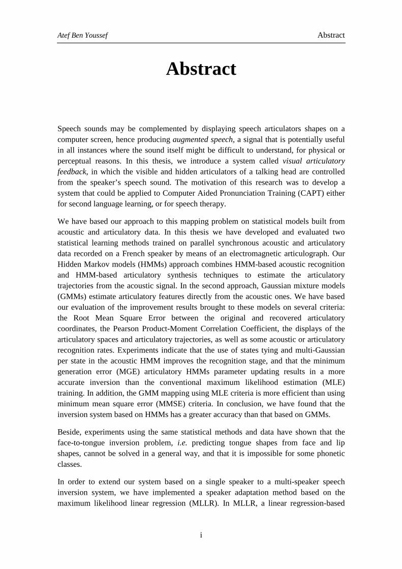
Speech sounds may be complemented by displaying speech articulators shapes on a computer screen, hence producing augmented speech, a signal that is potentially useful in all instances where the sound itself might be difficult to understand, for physical or perceptual reasons. In this thesis, we introduce a system called visual articulatory feedback, in which the visible and hidden articulators of a talking head are controlled from the speaker’s speech sound. The motivation of this research was to develop a system that could be applied to Computer Aided Pronunciation Training (CAPT) either for second language learning, or for speech therapy.
We have based our approach to this mapping problem on statistical models built from acoustic and articulatory data. In this thesis we have developed and evaluated two statistical learning methods trained on parallel synchronous acoustic and articulatory data recorded on a French speaker by means of an electromagnetic articulograph. Our Hidden Markov models (HMMs) approach combines HMM-based acoustic recognition and HMM-based articulatory synthesis techniques to estimate the articulatory trajectories from the acoustic signal. In the second approach, Gaussian mixture models (GMMs) estimate articulatory features directly from the acoustic ones. We have based our evaluation of the improvement results brought to these models on several criteria: the Root Mean Square Error between the original and recovered articulatory coordinates, the Pearson Product-Moment Correlation Coefficient, the displays of the articulatory spaces and articulatory trajectories, as well as some acoustic or articulatory recognition rates. Experiments indicate that the use of states tying and multi-Gaussian per state in the acoustic HMM improves the recognition stage, and that the minimum generation error (MGE) articulatory HMMs parameter updating results in a more accurate inversion than the conventional maximum likelihood estimation (MLE) training. In addition, the GMM mapping using MLE criteria is more efficient than using minimum mean square error (MMSE) criteria. In conclusion, we have found that the inversion system based on HMMs has a greater accuracy than that based on GMMs.
Beside, experiments using the same statistical methods and data have shown that the face-to-tongue inversion problem, i.e. predicting tongue shapes from face and lip shapes, cannot be solved in a general way, and that it is impossible for some phonetic classes.
In order to extend our system based on a single speaker to a multi-speaker speech inversion system, we have implemented a speaker adaptation method based on the maximum likelihood linear regression (MLLR). In MLLR, a linear regression-based
Atef Ben Youssef Abstract
ii
transform that adapts the original acoustic HMMs to those of the new speaker was calculated to maximise the likelihood of adaptation data. This speaker adaptation stage has been evaluated using an articulatory phonetic recognition system, as there are not original articulatory data available for the new speakers.
Finally, using this adaptation procedure, we have developed a complete articulatory feedback demonstrator, which can work for any speaker. This system should be assessed by perceptual tests in realistic conditions.
Keywords: visual articulatory feedback, acoustic-to-articulatory speech inversion mapping, ElectroMagnetic Articulography (EMA), hidden Markov models (HMMs), Gaussian mixture models (GMMs), speaker adaptation, face-to-tongue mapping
Atef Ben Youssef Résumé
iii
Résumé
Les sons de parole peuvent être complétés par l’affichage des articulateurs sur un écran d'ordinateur pour produire de la parole augmentée, un signal potentiellement utile dans tous les cas où le son lui-même peut être difficile à comprendre, pour des raisons physiques ou perceptuelles. Dans cette thèse, nous présentons un système appelé retour articulatoire visuel, dans lequel les articulateurs visibles et non visibles d’une tête parlante sont contrôlés à partir de la voix du locuteur. La motivation de cette thèse était de développer un système qui pourrait être appliqué à l’aide à l’apprentissage de la prononciation pour les langues étrangères, ou dans le domaine de l'orthophonie.
Nous avons basé notre approche de ce problème d’inversion sur des modèles statistiques construits à partir de données acoustiques et articulatoires enregistrées sur un locuteur français à l’aide d’un articulographe électromagnétique. Notre approche avec les modèles de Markov cachés (HMMs) combine des techniques de reconnaissance automatique de la parole et de synthèse articulatoire pour estimer les trajectoires articulatoires à partir du signal acoustique. D’un autre côté, les modèles de mélanges gaussiens (GMMs) estiment directement les trajectoires articulatoires à partir du signal acoustique sans faire intervenir d’information phonétique. Nous avons basé notre évaluation des améliorations apportées à ces modèles sur différents critères : l’erreur quadratique moyenne (RMSE) entre les trajectoires articulatoires originales et reconstruites, le coefficient de corrélation de Pearson, l’affichage des espaces et des trajectoires articulatoires, aussi bien que les taux de reconnaissance acoustique et articulatoire. Les expériences montrent que l’utilisation d'états liés et de multi-gaussiennes pour les états des HMMs acoustiques améliore l’étage de reconnaissance acoustique des phones, et que la minimisation de l'erreur générée (MGE) dans la phase d’apprentissage des HMMs articulatoires donne des résultats plus précis par rapport à l’utilisation du critère plus conventionnel de maximisation de vraisemblance (MLE). En outre, l’utilisation du critère MLE au niveau de mapping direct de l’acoustique vers l’articulatoire par GMMs est plus efficace que le critère de minimisation de l'erreur quadratique moyenne (MMSE). Nous avons également constaté que le système d'inversion par HMMs est plus précis celui basé sur les GMMs.
Par ailleurs, des expériences utilisant les mêmes méthodes statistiques et les mêmes données ont montré que le problème de reconstruction des mouvements de la langue à partir des mouvements du visage et des lèvres ne peut pas être résolu dans le cas général, et est impossible pour certaines classes phonétiques.
Atef Ben Youssef Résumé
iv
Afin de généraliser notre système basé sur un locuteur unique à un système d’inversion de parole multi-locuteur, nous avons implémenté une méthode d’adaptation du locuteur basée sur la maximisation de la vraisemblance par régression linéaire (MLLR). Dans cette méthode MLLR, la transformation basée sur la régression linéaire qui adapte les HMMs acoustiques originaux à ceux du nouveau locuteur est calculée de manière à maximiser la vraisemblance des données d’adaptation. Cet étage d’adaptation du locuteur a été évalué en utilisant un système de reconnaissance automatique des classes phonétiques de l’articulation, puisque les données articulatoires originales du nouveau locuteur n’existent pas.
Finalement, en utilisant cette procédure d'adaptation, nous avons développé un démonstrateur complet de retour articulatoire visuel, qui peut être utilisé par un locuteur quelconque. Ce système devra être évalué de manière perceptive dans des conditions réalistes.
Mots-clés : retour articulatoire visuel, inversion acoustique-articulatoire, articulographe électromagnétique, modèles de Markov cachées, modèles de mélanges gaussiens, adaptation au locuteur, inversion des mouvements faciaux vers les mouvements linguaux
Atef Ben Youssef Acknowledgement
v
Acknowledgement
First of all, I would like to express my sincere gratitude to my advisors Dr. Pierre Badin and Dr. Gérard Bailly, for their support, encouragement, and guidance during this thesis work.
Special thanks go to Prof. Jean-François Bonastre (LIA, Avignon, France) for accepting to be the president of the jury, to Dr. Yves Laprie (LORIA, Nancy, France) and Prof. Olov Engwall (KTH, Stockholm, Sweden) for accepting to evaluate my thesis as reviewers. I highly appreciated their detailed comments and remarks that greatly helped me to improve the quality of this manuscript.
I am grateful to Frederic Elisei, Christophe Savariaux, and Coriandre Vilain for their help in EMA recording.
I also wish to thank Thomas Hueber with whom I was fortunate to discuss and collaborate on the signal-to-signal mapping problem.
Thanks also to Viet-Anh Tran and Panikos Heracleous for their helpful discussions.
I would like to acknowledge my colleagues: Benjamin, Amélie, Sandra, Mathilde, Rosario and Hien for many good times with them during RJCP’2011 organisation.
Thanks to all the folk at GIPSA-Lab and special thanks go to all the members of Speech and Cognition Department.
I would sincerely like to thank my mother Naziha, my father Habib, my brothers Jihed, Nizar, Mourad, my sister Hanen, Ben Youssef’s family and my friends for their encouragement.
Finally, thanks to the Tunisian people "Leader of Arab Revolutions".

Atef Ben Youssef Content
vii
Content
Abstract .............................................................................................................................i
Résumé ............................................................................................................................ iii
Acknowledgement ............................................................................................................ v
Content .......................................................................................................................... vii
List of Figures .................................................................................................................xi
List of Tables .................................................................................................................. xv
Acronyms and terms ................................................................................................. xviii
Glossary .........................................................................................................................xix
Introduction ..................................................................................................................... 1
Chapter 1. Visual articulatory feedback in speech ....................................................... 5
1.1. Introduction ............................................................................................................ 5
1.2. Visual feedback devices ......................................................................................... 5
1.3. Talking head and augmented speech ..................................................................... 6
1.4. Visual feedback perception .................................................................................... 7
1.5. Visual feedback for phonetic correction ................................................................ 8
1.5.1. Speech Therapy .............................................................................................. 8
1.5.2. Language learning ........................................................................................ 10
1.6. Visual articulatory feedback system .................................................................... 11
1.7. Conclusion ........................................................................................................... 13
Chapter 2. Statistical mapping techniques for inversion ........................................... 15
2.1. Introduction .......................................................................................................... 15
2.2. Previous work ...................................................................................................... 15
2.2.1. Generative approach to inversion based on direct models ........................... 16
2.2.2. Statistical approach to inversion .................................................................. 18
2.2.3. Discussion .................................................................................................... 24
2.3. HMM-based speech recognition and synthesis ................................................... 24
2.3.1. Hidden Markov Models – General definitions............................................. 25
Atef Ben Youssef Content
viii
2.3.2. HMM Training ............................................................................................. 27 2.3.2.1 Multi-stream HMMs ........................................................................ 29
2.3.3. HMM-based inversion system ..................................................................... 30
2.3.4. Minimum Generation Error (MGE) training................................................ 32
2.3.5. Language models ......................................................................................... 34
2.4. GMM-based direct inversion ............................................................................... 36
2.4.1. Gaussian Mixture Models – General definitions ......................................... 36
2.4.2. GMM Training based on EM algorithm ...................................................... 36
2.4.3. GMM-based mapping using MMSE ............................................................ 38
2.4.4. GMM-based mapping using MLE ............................................................... 39
2.5. Summary .............................................................................................................. 42
Chapter 3. Acoustic and articulatory speech data ..................................................... 43
3.1. Introduction .......................................................................................................... 43
3.2. Methods for articulatory data acquisition ............................................................ 43
3.2.1. X-ray cineradiography ................................................................................. 43
3.2.2. X-ray microbeam cinematography ............................................................... 44
3.2.3. Magnetic Resonance Imaging ...................................................................... 44
3.2.4. Ultrasound echography ................................................................................ 44
3.2.5. ElectroMagnetic Articulography .................................................................. 45
3.2.6. Choice of articulatory data recording method .............................................. 45
3.3. Acoustic-articulatory corpuses ............................................................................ 47
3.3.1. EMA-PB-2007 corpus .................................................................................. 47 3.3.1.1 Phonetic content ............................................................................... 50
3.3.1.2 Statistic ............................................................................................ 50 3.3.1.3 Articulatory data validation ............................................................. 52
3.3.2. EMA-PB-2009 corpus .................................................................................. 56 3.3.2.1 Phonetic content ............................................................................... 56
3.3.2.2 Recording protocol .......................................................................... 56
3.3.2.3 Comparison between EMA-PB-2007 and EMA-PB-2009 .............. 57
3.3.3. MOCHA-TIMIT English corpus.................................................................. 61
3.4. Acoustic data for speaker adaptation ................................................................... 61
3.5. Acoustic and articulatory features extraction ...................................................... 62
3.6. Conclusion ........................................................................................................... 62
Chapter 4. Speech inversion evaluation ...................................................................... 65
4.1. Introduction .......................................................................................................... 65
Atef Ben Youssef Content
ix
4.2. Evaluation criteria ................................................................................................ 65
4.2.1. Train and test corpuses ................................................................................. 65
4.2.2. Measurements .............................................................................................. 67
4.2.3. Acoustic recognition .................................................................................... 68
4.2.4. Articulatory spaces ....................................................................................... 68
4.2.5. Articulatory recognition ............................................................................... 68 4.2.5.1 Method ............................................................................................. 68 4.2.5.2 Baseline ............................................................................................ 70
4.3. Evaluation results ................................................................................................. 73
4.3.1. HMM-based method .................................................................................... 73 4.3.1.1 Acoustic recognition ........................................................................ 73
4.3.1.2 Articulatory synthesis ...................................................................... 77
4.3.1.3 HMM-based results ......................................................................... 81
4.3.2. GMM-based method .................................................................................... 82 4.3.2.1 Impact of MLE for speech inversion mapping ................................ 84
4.3.2.2 GMM-based results ......................................................................... 84
4.4. Discussion ............................................................................................................ 86
4.5. Conclusion ........................................................................................................... 89
Chapter 5. Toward a multi-speaker visual articulatory feedback system ............... 93
5.1. Introduction .......................................................................................................... 93
5.2. Inversion based on Hidden Markov Models ........................................................ 94
5.3. Acoustic speaker adaptation ................................................................................ 95
5.4. Experiments and results ....................................................................................... 97
5.4.1. Articulatory recognition ............................................................................... 97
5.4.2. Evaluation of the predicted articulatory trajectories of new speakers ......... 97
5.4.3. Performances degradation when reducing the adaptation corpus size ......... 99
5.5. Visual articulatory feedback demonstrator ........................................................ 100
5.5.1. Animation of the talking head from EMA ................................................. 100
5.5.2. Demonstrator of the visual articulatory feedback system .......................... 101
5.6. Conclusion ......................................................................................................... 103
Chapter 6. Face-to-tongue mapping .......................................................................... 105
6.1. Introduction ........................................................................................................ 105
6.2. State-of-the-art ................................................................................................... 105
6.3. Evaluation .......................................................................................................... 107
6.3.1. Multi Linear Regression modeling............................................................. 107
Atef Ben Youssef Content
x
6.3.1.1 Evaluation of the MLR-based inversion ........................................ 108
6.3.2. HMM-based method .................................................................................. 108
6.3.3. GMM-based method .................................................................................. 109
6.4. Discussion .......................................................................................................... 109
6.5. Conclusion ......................................................................................................... 113
Chapter 7. Conclusions and perspectives .................................................................. 115
7.1. Conclusion ......................................................................................................... 115
7.2. Perspectives ....................................................................................................... 116
Bibliography ................................................................................................................. 121
Résumé en français de la thèse ................................................................................... 131
Publications .................................................................................................................. 151
Atef Ben Youssef List of Figures
xi
List of Figures
Figure 1.3-1. Augmented talking head for different types of display. Left: “augmented 2D view”, middle: “augmented 3D view”, right: “complete face in 3D with skin texture” ............................................................................................................................. 7
Figure 1.3-2. Illustration of the tongue body component of the 3D tongue model. Note the bunching (left) and the grooving (right) ..................................................................... 7
Figure 1.6-1. Schematic view of the articulatory feedback system for one speaker. ..... 12
Figure 1.6-2. Schematic view of the articulatory feedback system, where the speaker receives the feedback through the articulators of the teacher. ........................................ 13
Figure 2.2-1. Generative and statistical approaches used in previews work for speech inversion problem ........................................................................................................... 16
Figure 2.3-1. An example of hidden Markov models with 3 emitting states ................. 25
Figure 2.3-2. Matrix W of prediction of the sequence of static and dynamic features ( )yO as linear function of the static features by Y. Dy is the dimension of the static
vectors. ............................................................................................................................ 32
Figure 2.3-3. Overview of the acoustic-articulatory HMM-based speech inversion system combining two streams: acoustic for recognition and articulatory for synthesis. ........................................................................................................................................ 35
Figure 2.4-1. Overview of the GMM-based acoustic-to-articulatory speech inversion system ............................................................................................................................. 41
Figure 3.2-1. Picture of a subject’s tongue with three EMA coils attached to the tongue ........................................................................................................................................ 46
Figure 3.2-2. Illustration of the principle of the Electromagnetic articulograph: the transmitter and receiver coils positions are indicated ..................................................... 46
Figure 3.3-1. Positions of the six receiver coils attached to the lips, the jaw and the tongue (yellow dots). Positions of coils used as reference to correct the head movement (white dots). .................................................................................................................... 48
Atef Ben Youssef List of Figures
xii
Figure 3.3-2. Illustration of Parallel acoustic and articulatory signals for the sentence “Ma chemise est roussie” (phone boundaries are indicated by vertical bars – labels are indicated in the bottom frame)........................................................................................ 49
Figure 3.3-3. Average number of occurrences of each phoneme in the corpus EMA-PB-2007 ................................................................................................................................ 52
Figure 3.3-4. Dispersion ellipses of the measured coordinates of the six EMA coils for phoneme /t/. These ellipses are computed from the samples taken at the middle of the 231 instances of /t/ in the corpus. ................................................................................... 53
Figure 3.3-5. Dispersion ellipses of the measured coordinates of the six EMA coils for phoneme /k/. These ellipses are computed from the samples taken at the middle of the 130 instances of /k/ in the corpus. .................................................................................. 53
Figure 3.3-6. Confusion matrix of measured coordinates of the six EMA coils for vowels ............................................................................................................................. 54
Figure 3.3-7. Confusion tree of measured coordinates of the six EMA coils for vowels (the smaller the ordinate, the more confused the two categories are). The dashed line corresponds to a threshold level of 16 that leads to six classes. ..................................... 54
Figure 3.3-8. Confusion matrix of measured coordinates of the six EMA coils for consonants ...................................................................................................................... 55
Figure 3.3-9. Confusion tree of measured coordinates of the six EMA coils for consonants (the smaller the ordinate, the more confused the two categories are). The dashed line corresponds to a threshold level of 16 that leads to nine classes................. 55
Figure 3.3-10. Average number of occurrences of each phoneme in the corpus EMA-PB-2009 .......................................................................................................................... 58
Figure 3.3-11. Confusion matrix of vowels in EMA-PB-2009 corpus .......................... 59
Figure 3.3-12. Confusion tree of articulatory parameters of vowels in EMA-PB-2009 corpus (the smaller ordinate, the more confused the two categories are). The dashed line corresponds to a threshold level of 10 that leads to six classes. ..................................... 59
Figure 3.3-13. Confusion matrix of consonants in EMA-PB-2009 corpus .................... 60
Figure 3.3-14. Confusion tree of articulatory parameters of consonants in EMA-PB-2009 corpus (the smaller ordinate, the more confused the two categories are). The dashed line corresponds to a threshold level of 5 that leads to eleven classes. .............. 60
Figure 4.2-1. Distribution of number of occurrences for each phoneme of the five partitions of the EMA-PB-2007 corpus. ......................................................................... 66
Atef Ben Youssef List of Figures
xiii
Figure 4.2-2. Distribution of number of frames for each phoneme of the five partitions of the EMA-PB-2007. .................................................................................................... 66
Figure 4.2-3. Articulatory vowels clusters for speaker fsew0 ........................................ 72
Figure 4.2-4. Articulatory consonant clusters for speaker fsew0 ................................... 72
Figure 4.3-1. Articulatory spaces synthesised using MLE versus MGE trained models superposed on the measured articulatory space (grey contours, pertaining to midsagittal articulators contours for a consonant produced by the same speaker, are plotted here to serve as a reference frame) ............................................................................................. 80
Figure 4.3-2. Sample of synthesised Y-coordinates trajectories of an /aka/ sequence
using MGE and MLE trained models compared to the measured trajectories. .............. 80
Figure 4.4-1. Box plot, comparing HMM and GMM output, used to show the shape of the distribution, its central value, and variability. The graph produced consists of the most extreme values in the data set (maximum and minimum RMSE), the lower and upper quartiles, and the median. ..................................................................................... 86
Figure 4.4-2. Individual RMSEs for each phoneme. ...................................................... 87
Figure 4.4-3. Individual RMSEs for each EMA coil. ..................................................... 87
Figure 4.4-4. Articulatory spaces of the EMA coils for the phones sampled at centre. Black: measured coordinates; grey: synthesized coordinates. ....................................... 88
Figure 5.1-1. Different components of our visual articulatory feedback system ........... 94
Figure 5.4-1. Overview of multi-speaker inversion mapping and evaluation ................ 98
Figure 5.4-2. Influence of the corpus size on the acoustic adaptation performance .... 100
Figure 5.5-1. GIPSA-Lab’s talking head showing the articulators shapes with the EMA coils positions ............................................................................................................... 101
Figure 5.5-2. Top: Example of measured articulatory trajectories (thick line) and estimated using HMM-based mapping (thin line) from the audio speech alone for the VCV [ɛkɛ] (only tongue EMA coils are displayed). Bottom: Corresponding animation of the talking head (only one frame per phoneme is displayed). .................................. 102
Figure 6.4-1. Dispersion ellipses of coils for phones with errors larger than 10 mm for at least one coil coordinate: original data (thick lines), estimated data (thin lines), superposed on original data points for all phones (light grey dots). Note the general backing of the estimates. .............................................................................................. 110

Atef Ben Youssef List of Figures
xiv
Figure 6.4-2. Confusion matrices of the tongue phoneme estimated from facial movement using three mapping approach on EMA-PB-2007 corpus .......................... 112
Figure 7.2-1. Evaluation of the generalisation capacity of the HMM-based method .. 118
Atef Ben Youssef List of Tables
xv
List of Tables
Table 3.2-1 Comparison of 5 speech articulation measurement systems (modified from (Ridouane, 2006)) ........................................................................................................... 47
Table 3.3-1. Possible French allophones ........................................................................ 51
Table 3.3-2. Comparison between EMA-PB-2007 and EMA-PB-2009 corpuses ......... 57
Table 3.3-3. Comparison between the two French corpuses and the English one ......... 61
Table 3.4-1. Statistic of the three audio corpuses (* indicate the reference speaker who record EMA-PB-2007 corpus) ....................................................................................... 62
Table 4.2-1. Articulatory phoneme classes used to train the articulatory models and to recognise the articulatory trajectories ............................................................................. 69
Table 4.2-2. Articulatory recognition rates of the measured trajectories of EMA-PB-2007 corpus (percent correct and accuracy) ................................................................... 71
Table 4.2-3. Articulatory recognition rates of the measured trajectories of EMA-PB-2009 corpus .................................................................................................................... 71
Table 4.2-4. Articulatory recognition rates of the measured trajectories of MOCHA-TIMIT corpus ................................................................................................................. 73
Table 4.3-1. Recognition rates (Percent Correct, Accuracy) aggregated over the whole EMA-PB-2007 corpus .................................................................................................... 73
Table 4.3-2. Recognition rates using inheritance mechanism aggregated over the whole EMA-PB-2007 corpus .................................................................................................... 74
Table 4.3-3. Recognition rates (Percent Correct, Accuracy) aggregated over the whole EMA-PB-2007 corpus as a function of number of Gaussians. The rates of states reducing (tied-states) are about 55%, 57% and 63% for L-ctx, ctx-R and L-ctx-R, respectively. .................................................................................................................... 75
Table 4.3-4. Influence of parameterisation on recognition performance on the EMA-PB-2007 corpus .................................................................................................................... 76
Table 4.3-5. Impact of the language model on recognition performance on the EMA-PB-2007 corpus .............................................................................................................. 76
Atef Ben Youssef List of Tables
xvi
Table 4.3-6. Inversion performances using the MLE training method on the EMA-PB-2007 corpus .................................................................................................................... 77
Table 4.3-7. Influence of state duration prediction on the performance of the articulatory synthesis stage using MLE trained models on the EMA-PB-2007 corpus .................... 78
Table 4.3-8. Performances of MLE and MGE trained model on the EMA-PB-2007 corpus using a perfect recognition stage......................................................................... 79
Table 4.3-9. Performances of the full inversion using MGE trained models on the EMA-PB-2007 corpus .............................................................................................................. 79
Table 4.3-10. HMM-based inversion performances of the French EMA-PB-2009 and the English MOCHA-TIMIT corpuses ........................................................................... 82
Table 4.3-11. Inversion performances of the MMSE-based mapping as a function of number of Gaussians (# mix) and of context size (ms). ................................................. 83
Table 4.3-12. Inversion result of MLE-based mapping as a function of number of Gaussians (# mix) and size of context (ms). ................................................................... 84
Table 4.3-13. Inversion performance of the GMM-based mapping using MLE on EMA-PB-2009 and MOCHA-TIMIT corpus ........................................................................... 85
Table 4.5-1 Comparison of inversion results (µRMSE) found in the literature. * indicates that µRMSE was found using the same data set as Richmond (2002): files whose numbers end with 2 for validation (46 utterances), those ending with 6 for testing (46 utterances) and the remaining 368 utterances for training. ...................................... 90
Table 5.2-1. Performances of the HMM-based inversion using 1/5 of the EMA-PB-2007 corpus for testing. ........................................................................................................... 95
Table 5.4-1. Articulatory recognition rates of the measured trajectories of the remaining fifth partition of the EMA-PB-2007 corpus (percent correct and accuracy) .................. 97
Table 5.4-2. Acoustic and articulatory recognition accuracy for all the speakers, using 1/5 of the corpus for testing. ........................................................................................... 99
Table 6.2-1. Correlation coefficients for each EMA coordinate (bold for maximum and italics for minimum values) for the various studies. .................................................... 107
Table 6.3-1. RMSE (mm) and PMCC for the HMM inversion with different types of contexts. ........................................................................................................................ 108
Table 6.3-2 Recognition rates (Percent Correct, Accuracy) for phoneme recognition from Face and phoneme recognition from Acoustics. .................................................. 109

Atef Ben Youssef List of Tables
xvii
Table 6.3-3. RMSE (mm) and PMCC for the GMM inversion (MLE) with different numbers of mixtures (# mix) and context window sizes (ctw). ................................... 109
Table 6.4-1. RMSE for individual phonemes (mm). .................................................... 110
Atef Ben Youssef Acronyms and terms
xviii
Acronyms and terms
ANN Artificial Neural Network
ASR Automatic Speech Recognition
CAPT Computer Aided Pronunciation Training
CVC Consonant-Vowel- Consonant
EM Expectation Maximisation
EMA ElectroMagnetic Articulography
GMM Gaussian Mixture Model
HMM Hidden Markov Model
L1 First language or mother tongue
L2 Second Language; Foreign Language
MFCC Mel-Frequency Cepstral coefficients
MGE Minimum Generation Error
MLE Maximum Likelihood Estimation
MLLR Maximum Likelihood Linear Regression
MLP Multi-Layer Perceptron
MLPG Maximum-Likelihood Parameter Generation
MLR Multi Linear Regression
MMSE Minimum Mean-Square Error
MRI Magnetic Resonance Imaging
PCA Principal Analysis Component
PDF Probability Density Function
PMCC Pearson Product-Moment Correlation Coefficient
RMSE/RMS error Root Mean Square Error
SVMs Support Vector Machines
TTS Text-To-Speech synthesis
VCV Vowel-Consonant-Vowel
VTH Virtual Talking Head
Atef Ben Youssef Glossary
xix
Glossary
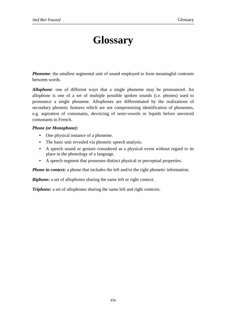
Phoneme: the smallest segmental unit of sound employed to form meaningful contrasts between words.
Allophone: one of different ways that a single phoneme may be pronounced. An allophone is one of a set of multiple possible spoken sounds (i.e. phones) used to pronounce a single phoneme. Allophones are differentiated by the realizations of secondary phonetic features which are not compromising identification of phonemes, e.g. aspiration of consonants, devoicing of semi-vowels or liquids before unvoiced consonants in French.
Phone (or Monophone):
• One physical instance of a phoneme.
• The basic unit revealed via phonetic speech analysis.
• A speech sound or gesture considered as a physical event without regard to its place in the phonology of a language.
• A speech segment that possesses distinct physical or perceptual properties.
Phone in context: a phone that includes the left and/or the right phonetic information.
Biphone: a set of allophones sharing the same left or right context.
Triphone: a set of allophones sharing the same left and right contexts.

Introduction
1
Introduction
Motivation of research
“Speech is rather a set of movements made audible than a set of sounds produced by movements” (Stetson, 1928). This statement means that speech is not only sounds which are produced just to be heard but it can also be regarded as visible signals resulting from articulatory movement. Therefore, speech sound may be complemented or augmented with visible signals (simple video, display of usually hidden articulators such as tongue or velum, hand gestures as used in cued speech by hearing-impaired people, etc.). Augmented speech may offer very fruitful potentialities in various speech communication situations where the audio signal itself is degraded (noisy environment, impairment hearing, etc.), or in the domain of speech rehabilitation (speech therapy, phonetic correction, etc.).
Visual articulatory feedback systems aim at providing the speaker with visual information about his/her own articulation: the view of visible articulators, i.e. jaw and lips, improves speech intelligibility (Sumby and Pollack, 1954), speech imitation is faster when listeners perceive articulatory gestures (Fowler et al., 2003), and the vision of hidden articulators still increases intelligibility (Badin et al., 2010).
The overall objective of this thesis was thus to develop inversion tools and to design and implement a system that allows producing augmented speech from the speech sound signal alone, and to use it to build a visual articulatory feedback system that may be used in Computer Aided Pronunciation Training (CAPT) or for speech rehabilitation.
The main difficulty is that there is no one-to-one mapping between the acoustic and articulatory domains and there are thus a large number of vocal tract shapes that can produce the same speech signal (Atal et al., 1978). Indeed, the problem is under-determined, as there are more unknowns that need to be determined than input data available.
Speech inversion was traditionally based on model-based analysis-by-synthesis. One important issue was to add constraints (contextual, linguistic...) that are both sufficiently restrictive and realistic from a phonetic point of view, in order to eliminate sub-optimal solutions. But since a decade, more sophisticated data-driven techniques have appeared, thanks to the availability of large corpora of articulatory and acoustic data provided by devices such as the ElectroMagnetic Articulograph (EMA) or motion tracking devices based on classical or infrared video. The medical imaging techniques for obtaining
Introduction
2
vocal tract deformation are sufficiently nature to provide massive articulatory data that can be exploited for helping both the design and the evaluation of data-driven inversion methods. Besides, statistical modelling have now reached a sufficient maturity to envisage their applications to real systems.
Organization of the manuscript
The thesis manuscript is organised as follows.
Chapter 1 introduces the aim of visual articulatory feedback and presents devices that are able to provide it, followed by the presentation of the talking head developed in GIPSA-Lab. This interface can animate the visible and hidden articulators using ElectroMagnetic Articulography (EMA). Finally, we present the different potential uses of the visual articulatory feedback system.
Chapter 2 provides background information on articulatory feedback production and perception from previous research. This chapter starts with the previous work on acoustic-to-articulatory speech inversion based on physical modelling versus statistical modelling. Then, we describe two statistical approaches that we used: the first approach is based on hidden Markov models (HMM) and the second one is based on Gaussian mixture models (GMM).
Chapter 3 focuses on the acquisition and the description of our parallel acoustic and articulatory data. The chapter presents the construction of the French corpuses recorded by one male French speaker using EMA. A comparison between our French corpus and an English corpus (MOCHA-TIMIT) is also presented in this chapter. Three audio corpuses recorded by two males and a female French native speaker are then described. These corpuses have been used for the acoustic speaker adaptation. The acoustic and articulatory parameterisation is presented in the end of this chapter.
Chapter 4 describes the evaluation criteria used to evaluate the HMM- and GMM-based methods. The results that include the improvement of the described methods are presented and discussed. The improvement of the HMM-based method is mainly due to state tying, the increase of the number of Gaussians in the acoustic stream and the training of the articulatory stream using the Minimum Generation Error (MGE) criterion. The improvement of the GMM-based method is based on the use of MLE mapping method instead of MMSE one. Next, we discussed the best results of the HMM and GMM.
Chapter 5 describes the adaptation of the acoustic HMMs of the “reference speaker” to the new speaker’s voice using the Maximum Likelihood Linear Regression (MLLR) technique. Then, we evaluate this stage on three audio corpuses described above. Finally, we describe the prototype of the visual articulatory feedback system that we have developed.
Introduction
3
Chapter 6 presents the face-to-tongue mapping debate found in the literature. In this chapter, we applied the same techniques and corpus used for speech inversion to evaluate the reconstruction of tongue shape from face shape.
Finally, Chapter 7 presents the conclusions that summarize the contributions of this thesis and discusses suggestions for future work.
Note: related project ARTIS
Note that the work presented in this thesis contributed to the French ANR-08-EMER-001-02 ARTIS project which involves collaboration between GIPSA-Lab, LORIA, ENST-Paris and IRIT. The main objective of this research project is to provide augmented speech with visible and hidden articulators by means of a virtual talking head from the speech sound signal alone or with video images of the speaker’s face.

Chapter 1. Visual articulatory feedback in speech
5
Chapter 1. Visual articulatory feedback in speech
1.1. Introduction
It has become common sense to say that speech is not merely an acoustic signal but a signal endowed with complementary coherent traces such as visual, tactile or physiological signals (Bailly et al., 2010).
Besides, it has been demonstrated that humans possess – to some degree – articulatory awareness skills, as evidenced e.g. by Montgomery (1981) or Thomas & Sénéchal (1998). These results support the hypothesis that accuracy of articulation is related to quality of phoneme awareness in young children, while Kröger et al. (2008) found that children older than five years are capable to produce the articulators positions displayed using an articulatory model without any preparatory training in a speech adequate way. Finally, Badin et al (2010) have recently demonstrated that human subjects are able – to some extent – to make use of tongue shape vision for phonemic recognition, as they do with lips in lip reading. All these findings suggest that visual articulatory feedback could help subjects acquire the articulatory strategies needed to produce sounds that are new to them.
In the present chapter, we describe devices that are able to provide a visual articulatory feedback in section 1.2. In section 1.3, we present a talking head that can produce speech augmented by the display of hidden articulators. Section 1.4 presents the impact of tongue visualisation on speech perception; while the section 1.5 presents the state-of-the-art in the domain of visual feedback for phonetic correction and section 1.6 discusses a general framework for a visual articulatory feedback system.
1.2. Visual feedback devices
Several devices are able to provide information on the movements of visible and hidden articulators. The mirror is the much more basic way of providing feedback of visible articulators, (i.e. jaw and lips) by showing in real-time the speaker’s face movement. Moreover, face movement can also be displayed in real-time or not using simple video recorded by camera. Concerning hidden articulators, many techniques provide partial information of the inner speech organs in motion:
Chapter 1. Visual articulatory feedback in speech
6
• ElectroPalatoGraphy (EPG) provides real-time visual feedback of the location and timing of tongue contacts with the hard palate during speech.
• Ultrasound imaging provides a visual feedback by showing a partial 2D surface of the tongue.
• ElectroMagnetic Articulography (EMA) provides 2D or 3D movements of a few coils attached to the tongue or other articulators, including the velum, with high precision.
These techniques are complex to implement, expensive and esoteric. Our aim is to develop a new technique of visual articulatory feedback via virtual talking head that provide augmented speech and could be used by any speaker easily.
1.3. Talking head and augmented speech
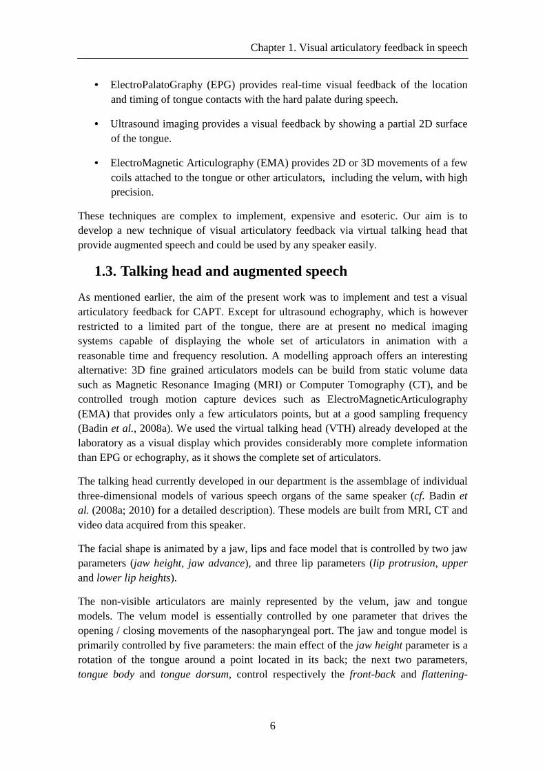
As mentioned earlier, the aim of the present work was to implement and test a visual articulatory feedback for CAPT. Except for ultrasound echography, which is however restricted to a limited part of the tongue, there are at present no medical imaging systems capable of displaying the whole set of articulators in animation with a reasonable time and frequency resolution. A modelling approach offers an interesting alternative: 3D fine grained articulators models can be build from static volume data such as Magnetic Resonance Imaging (MRI) or Computer Tomography (CT), and be controlled trough motion capture devices such as ElectroMagneticArticulography (EMA) that provides only a few articulators points, but at a good sampling frequency (Badin et al., 2008a). We used the virtual talking head (VTH) already developed at the laboratory as a visual display which provides considerably more complete information than EPG or echography, as it shows the complete set of articulators.
The talking head currently developed in our department is the assemblage of individual three-dimensional models of various speech organs of the same speaker (cf. Badin et al. (2008a; 2010) for a detailed description). These models are built from MRI, CT and video data acquired from this speaker.
The facial shape is animated by a jaw, lips and face model that is controlled by two jaw parameters (jaw height, jaw advance), and three lip parameters (lip protrusion, upper and lower lip heights).
The non-visible articulators are mainly represented by the velum, jaw and tongue models. The velum model is essentially controlled by one parameter that drives the opening / closing movements of the nasopharyngeal port. The jaw and tongue model is primarily controlled by five parameters: the main effect of the jaw height parameter is a rotation of the tongue around a point located in its back; the next two parameters, tongue body and tongue dorsum, control respectively the front-back and flattening-
Chapter 1. Visual articulatory feedback in speech
7
arching movements of the tongue; the last other two parameters, tongue tip vertical and tongue tip horizontal control precisely the shape of the tongue tip (Badin & Serrurier, 2006).
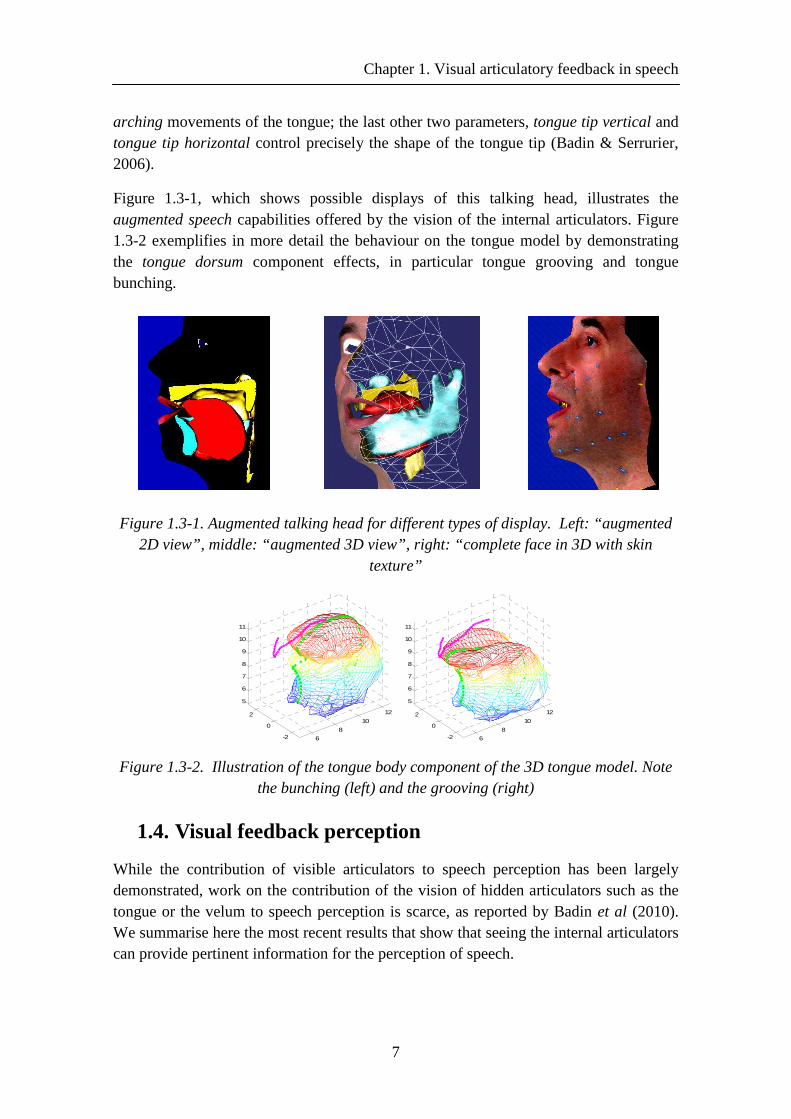
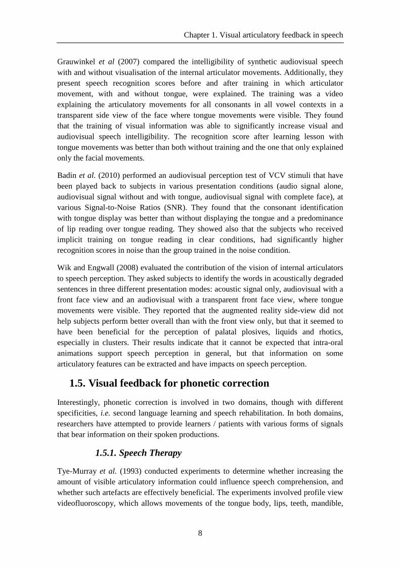
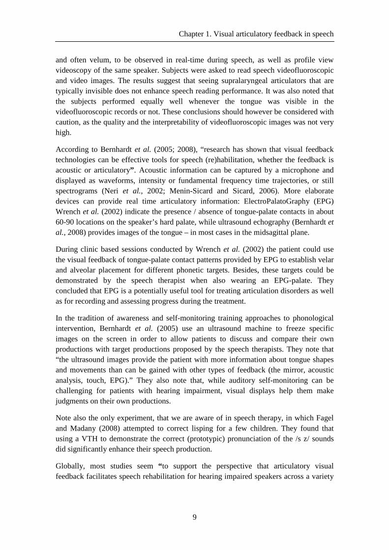
Figure 1.3-1, which shows possible displays of this talking head, illustrates the augmented speech capabilities offered by the vision of the internal articulators. Figure 1.3-2 exemplifies in more detail the behaviour on the tongue model by demonstrating the tongue dorsum component effects, in particular tongue grooving and tongue bunching.
Figure 1.3-1. Augmented talking head for different types of display. Left: “augmented 2D view”, middle: “augmented 3D view”, right: “complete face in 3D with skin
texture”
6
8
10
12
-2
0
2
5
6
7
8
9
10
11
6
8
10
12
-2
0
2
5
6
7
8
9
10
11
Figure 1.3-2. Illustration of the tongue body component of the 3D tongue model. Note the bunching (left) and the grooving (right)
1.4. Visual feedback perception
While the contribution of visible articulators to speech perception has been largely demonstrated, work on the contribution of the vision of hidden articulators such as the tongue or the velum to speech perception is scarce, as reported by Badin et al (2010). We summarise here the most recent results that show that seeing the internal articulators can provide pertinent information for the perception of speech.
Chapter 1. Visual articulatory feedback in speech
8
Grauwinkel et al (2007) compared the intelligibility of synthetic audiovisual speech with and without visualisation of the internal articulator movements. Additionally, they present speech recognition scores before and after training in which articulator movement, with and without tongue, were explained. The training was a video explaining the articulatory movements for all consonants in all vowel contexts in a transparent side view of the face where tongue movements were visible. They found that the training of visual information was able to significantly increase visual and audiovisual speech intelligibility. The recognition score after learning lesson with tongue movements was better than both without training and the one that only explained only the facial movements.
Badin et al. (2010) performed an audiovisual perception test of VCV stimuli that have been played back to subjects in various presentation conditions (audio signal alone, audiovisual signal without and with tongue, audiovisual signal with complete face), at various Signal-to-Noise Ratios (SNR). They found that the consonant identification with tongue display was better than without displaying the tongue and a predominance of lip reading over tongue reading. They showed also that the subjects who received implicit training on tongue reading in clear conditions, had significantly higher recognition scores in noise than the group trained in the noise condition.
Wik and Engwall (2008) evaluated the contribution of the vision of internal articulators to speech perception. They asked subjects to identify the words in acoustically degraded sentences in three different presentation modes: acoustic signal only, audiovisual with a front face view and an audiovisual with a transparent front face view, where tongue movements were visible. They reported that the augmented reality side-view did not help subjects perform better overall than with the front view only, but that it seemed to have been beneficial for the perception of palatal plosives, liquids and rhotics, especially in clusters. Their results indicate that it cannot be expected that intra-oral animations support speech perception in general, but that information on some articulatory features can be extracted and have impacts on speech perception.
1.5. Visual feedback for phonetic correction
Interestingly, phonetic correction is involved in two domains, though with different specificities, i.e. second language learning and speech rehabilitation. In both domains, researchers have attempted to provide learners / patients with various forms of signals that bear information on their spoken productions.
1.5.1. Speech Therapy
Tye-Murray et al. (1993) conducted experiments to determine whether increasing the amount of visible articulatory information could influence speech comprehension, and whether such artefacts are effectively beneficial. The experiments involved profile view videofluoroscopy, which allows movements of the tongue body, lips, teeth, mandible,
Chapter 1. Visual articulatory feedback in speech
9
and often velum, to be observed in real-time during speech, as well as profile view videoscopy of the same speaker. Subjects were asked to read speech videofluoroscopic and video images. The results suggest that seeing supralaryngeal articulators that are typically invisible does not enhance speech reading performance. It was also noted that the subjects performed equally well whenever the tongue was visible in the videofluoroscopic records or not. These conclusions should however be considered with caution, as the quality and the interpretability of videofluoroscopic images was not very high.
According to Bernhardt et al. (2005; 2008), “research has shown that visual feedback technologies can be effective tools for speech (re)habilitation, whether the feedback is acoustic or articulatory” . Acoustic information can be captured by a microphone and displayed as waveforms, intensity or fundamental frequency time trajectories, or still spectrograms (Neri et al., 2002; Menin-Sicard and Sicard, 2006). More elaborate devices can provide real time articulatory information: ElectroPalatoGraphy (EPG) Wrench et al. (2002) indicate the presence / absence of tongue-palate contacts in about 60-90 locations on the speaker’s hard palate, while ultrasound echography (Bernhardt et al., 2008) provides images of the tongue – in most cases in the midsagittal plane.
During clinic based sessions conducted by Wrench et al. (2002) the patient could use the visual feedback of tongue-palate contact patterns provided by EPG to establish velar and alveolar placement for different phonetic targets. Besides, these targets could be demonstrated by the speech therapist when also wearing an EPG-palate. They concluded that EPG is a potentially useful tool for treating articulation disorders as well as for recording and assessing progress during the treatment.
In the tradition of awareness and self-monitoring training approaches to phonological intervention, Bernhardt et al. (2005) use an ultrasound machine to freeze specific images on the screen in order to allow patients to discuss and compare their own productions with target productions proposed by the speech therapists. They note that “the ultrasound images provide the patient with more information about tongue shapes and movements than can be gained with other types of feedback (the mirror, acoustic analysis, touch, EPG).” They also note that, while auditory self-monitoring can be challenging for patients with hearing impairment, visual displays help them make judgments on their own productions.
Note also the only experiment, that we are aware of in speech therapy, in which Fagel and Madany (2008) attempted to correct lisping for a few children. They found that using a VTH to demonstrate the correct (prototypic) pronunciation of the /s z/ sounds did significantly enhance their speech production.
Globally, most studies seem “ to support the perspective that articulatory visual feedback facilitates speech rehabilitation for hearing impaired speakers across a variety
Chapter 1. Visual articulatory feedback in speech
10
of sound classes by providing information about tongue contact, movement, and shape” (Bernhardt et al., 2003).
1.5.2. Language learning
Oppositely to speech therapy, most of the literature in Computer Aided Pronunciation Training (CAPT) seems to deal visual feedback that does not involve explicit articulatory information. Menzel et al. (2001) mention that “usually, a simple playback facility along with a global scoring mechanism and a visual presentation of the signal form or some derived parameters like pitch are provided.” But they pinpoint that a crucial task is left to the student, i.e. identifying the place and the nature of the pronunciation problem. According to them, automatic speech recognition (ASR) is often used to localise the errors, and even to perform an analysis in terms of phone substitutions, insertions or omissions, as well as in terms of misplaced word stress patterns. But they note that, while the “feedback is provided to the student through a multimedia-based interface, all the interaction is carried out using only the orthographic representations”. Though more and more precise and flexible ASR systems have allowed progress in CAPT (Chun, 2007; Cucchiarini et al., 2009), it may be interesting to explore the potentialities of visual articulatory feedback.
A limited but interesting series of studies has used virtual talking heads (VTH) controlled by text-to-speech synthesis to display speech articulators – including usually hidden ones such as the tongue. These displays are meant to demonstrate targets for helping learners acquiring new or correct articulations, though they actually do not provide a real feedback of the learner’s articulators as in speech therapy.
Massaro & Light (2004) found that using a VTH as a language tutor for children with hearing loss lead to some quantitative improvement of their performances. Later, using the same talking head, Massaro et al. (2008) showed that visible speech could contribute positively to the acquisition of new speech distinctions and promoting active learning, though they could not conclude about the effectiveness of showing internal articulatory movements for pronunciation training.
Engwall (2008) implemented an indirect visual articulatory feedback by means of a wizard-of-Oz set-up, in which an expert phonetician chose the adequate pre-generated feedback with a VTH meant to guide the learner to produce the right articulation. He found that this helped French subjects improve their pronunciation of Swedish words, though he did not perform any specific evaluation of the benefit of the vision of the tongue.
Other studies investigated the visual information conveyed by the vision of internal articulators.
Chapter 1. Visual articulatory feedback in speech
11
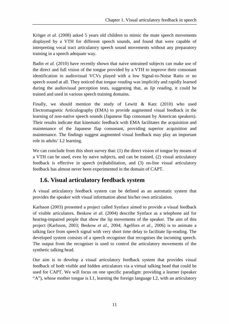
Kröger et al. (2008) asked 5 years old children to mimic the mute speech movements displayed by a VTH for different speech sounds, and found that were capable of interpreting vocal tract articulatory speech sound movements without any preparatory training in a speech adequate way.
Badin et al. (2010) have recently shown that naive untrained subjects can make use of the direct and full vision of the tongue provided by a VTH to improve their consonant identification in audiovisual VCVs played with a low Signal-to-Noise Ratio or no speech sound at all. They noticed that tongue reading was implicitly and rapidly learned during the audiovisual perception tests, suggesting that, as lip reading, it could be trained and used in various speech training domains.
Finally, we should mention the study of Lewitt & Katz (2010) who used Electromagnetic Articulography (EMA) to provide augmented visual feedback in the learning of non-native speech sounds (Japanese flap consonant by American speakers). Their results indicate that kinematic feedback with EMA facilitates the acquisition and maintenance of the Japanese flap consonant, providing superior acquisition and maintenance. The findings suggest augmented visual feedback may play an important role in adults’ L2 learning.
We can conclude from this short survey that: (1) the direct vision of tongue by means of a VTH can be used, even by naive subjects, and can be trained, (2) visual articulatory feedback is effective in speech (re)habilitation, and (3) on-line visual articulatory feedback has almost never been experimented in the domain of CAPT.
1.6. Visual articulatory feedback system
A visual articulatory feedback system can be defined as an automatic system that provides the speaker with visual information about his/her own articulation.
Karlsson (2003) presented a project called Synface aimed to provide a visual feedback of visible articulators. Beskow et al. (2004) describe Synface as a telephone aid for hearing-impaired people that show the lip movements of the speaker. The aim of this project (Karlsson, 2003; Beskow et al., 2004; Agelfors et al., 2006) is to animate a talking face from speech signal with very short time delay to facilitate lip-reading. The developed system consists of a speech recogniser that recognises the incoming speech. The output from the recogniser is used to control the articulatory movements of the synthetic talking head.
Our aim is to develop a visual articulatory feedback system that provides visual feedback of both visible and hidden articulators via a virtual talking head that could be used for CAPT. We will focus on one specific paradigm: providing a learner (speaker “A”), whose mother tongue is L1, learning the foreign language L2, with an articulatory
Chapter 1. Visual articulatory feedback in speech
12
feedback displayed by means of the talking head of the teacher (speaker “B”) who is supposed to be bilingual in L1 and L2.
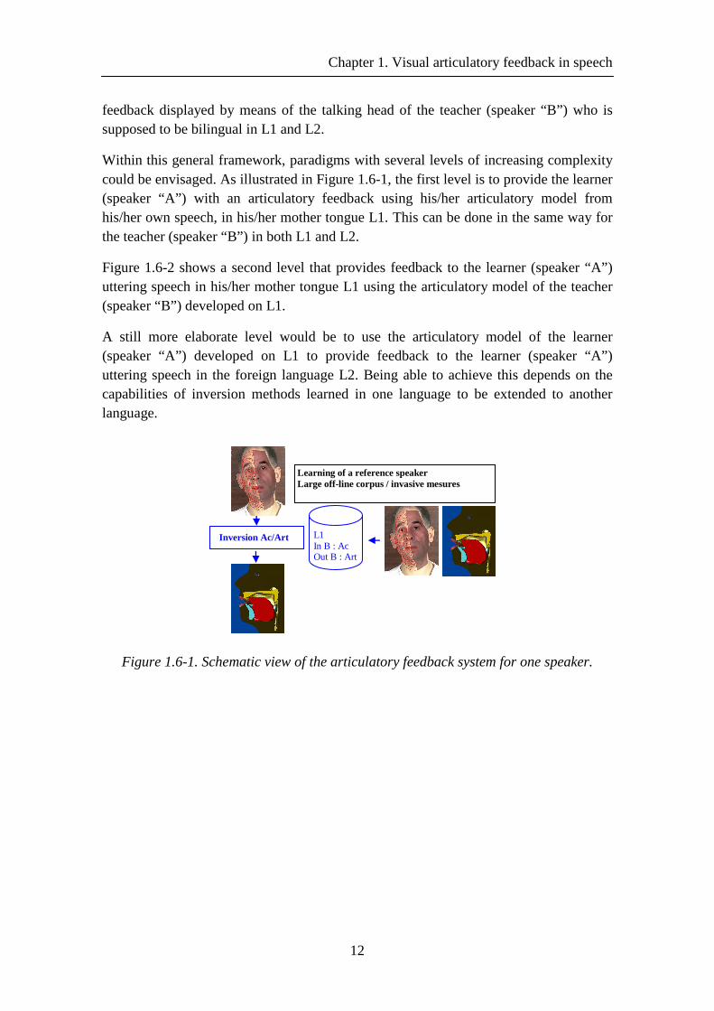
Within this general framework, paradigms with several levels of increasing complexity could be envisaged. As illustrated in Figure 1.6-1, the first level is to provide the learner (speaker “A”) with an articulatory feedback using his/her articulatory model from his/her own speech, in his/her mother tongue L1. This can be done in the same way for the teacher (speaker “B”) in both L1 and L2.
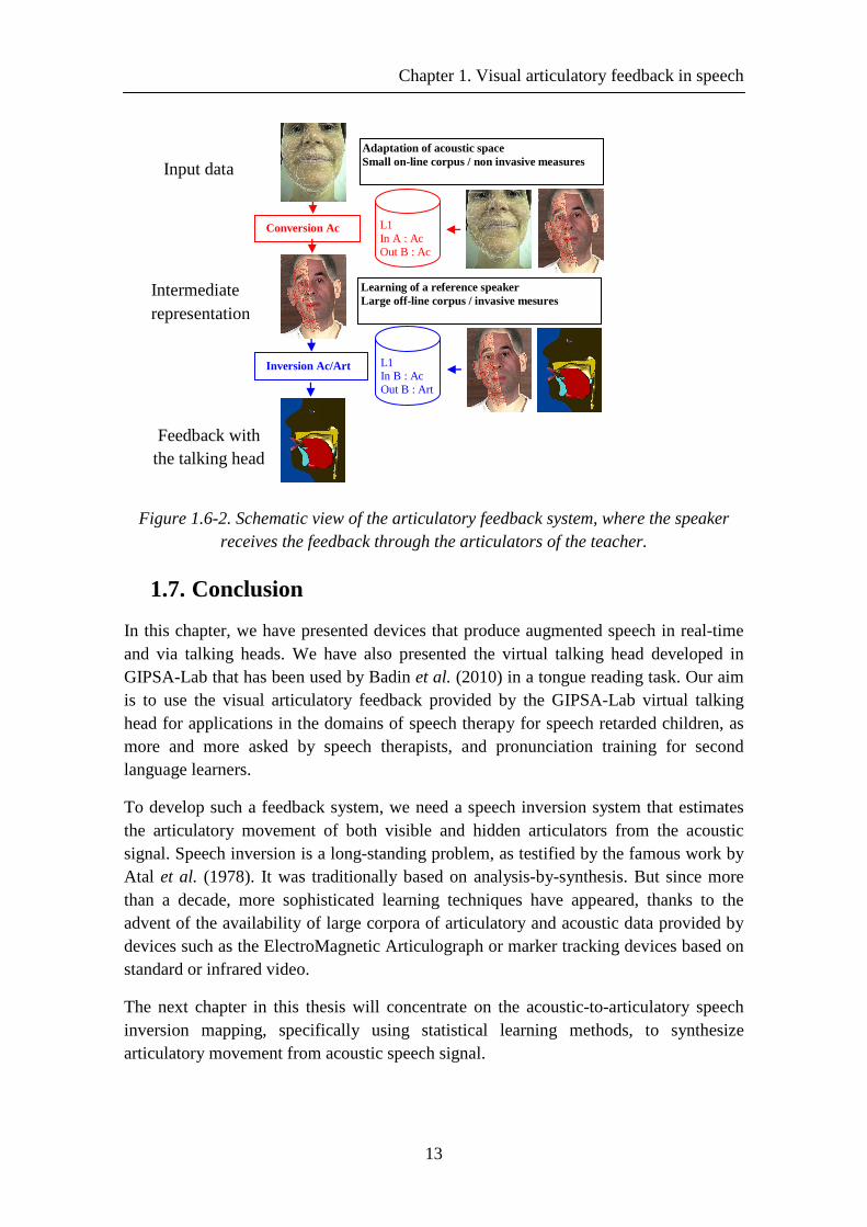
Figure 1.6-2 shows a second level that provides feedback to the learner (speaker “A”) uttering speech in his/her mother tongue L1 using the articulatory model of the teacher (speaker “B”) developed on L1.
A still more elaborate level would be to use the articulatory model of the learner (speaker “A”) developed on L1 to provide feedback to the learner (speaker “A”) uttering speech in the foreign language L2. Being able to achieve this depends on the capabilities of inversion methods learned in one language to be extended to another language.
L1 In B : Ac Out B : Art
Inversion Ac/Art
Learning of a reference speaker Large off-line corpus / invasive mesures
Figure 1.6-1. Schematic view of the articulatory feedback system for one speaker.
Chapter 1. Visual articulatory feedback in speech
13
L1 In A : Ac Out B : Ac
Conversion Ac
L1 In B : Ac Out B : Art
Inversion Ac/Art
Adaptation of acoustic space Small on-line corpus / non invasive measures
Learning of a reference speaker Large off-line corpus / invasive mesures
Figure 1.6-2. Schematic view of the articulatory feedback system, where the speaker receives the feedback through the articulators of the teacher.
1.7. Conclusion
In this chapter, we have presented devices that produce augmented speech in real-time and via talking heads. We have also presented the virtual talking head developed in GIPSA-Lab that has been used by Badin et al. (2010) in a tongue reading task. Our aim is to use the visual articulatory feedback provided by the GIPSA-Lab virtual talking head for applications in the domains of speech therapy for speech retarded children, as more and more asked by speech therapists, and pronunciation training for second language learners.
To develop such a feedback system, we need a speech inversion system that estimates the articulatory movement of both visible and hidden articulators from the acoustic signal. Speech inversion is a long-standing problem, as testified by the famous work by Atal et al. (1978). It was traditionally based on analysis-by-synthesis. But since more than a decade, more sophisticated learning techniques have appeared, thanks to the advent of the availability of large corpora of articulatory and acoustic data provided by devices such as the ElectroMagnetic Articulograph or marker tracking devices based on standard or infrared video.
The next chapter in this thesis will concentrate on the acoustic-to-articulatory speech inversion mapping, specifically using statistical learning methods, to synthesize articulatory movement from acoustic speech signal.
Input data
Feedback with the talking head
Intermediate representation

Chapter 2. Statistical mapping techniques for inversion
15
Chapter 2. Statistical mapping techniques for inversion
2.1. Introduction
In Chapter 1, we have presented a visual articulatory feedback system for speech training and rehabilitation. The present chapter concentrates on the development of such a feedback system. Chapter 2 aims to present the different approaches to the problem of estimation of the articulatory movements from the acoustic signal, also known as speech inversion or acoustic-to-articulatory mapping. To date, studies on the mapping between acoustic signal and articulatory signal found in the literature are based on either physical models or statistical models of the articulatory-to-acoustic relation. The goal of Chapter 2 is to review the major studies on acoustic-to-articulatory speech inversion of literature, and to describe in particular two statistical approaches. The first approach is based on Hidden Markov Models (HMMs), which are traditionally used in Automatic Speech Recognition (ASR) and Text To Speech (TTS) synthesis. Then, the second approach is based on Gaussian Mixture Models (GMMs) used usually in voice conversion.
The chapter is organized as follows. Section 2.2 reviews the literature on speech inversion. Section 2.3 provides an overview of the multi-stream HMM-based acoustic phone recognition and articulatory phone synthesis system. Section 2.4 describes the GMM-based direct acoustic-to-articulatory mapping.
2.2. Previous work
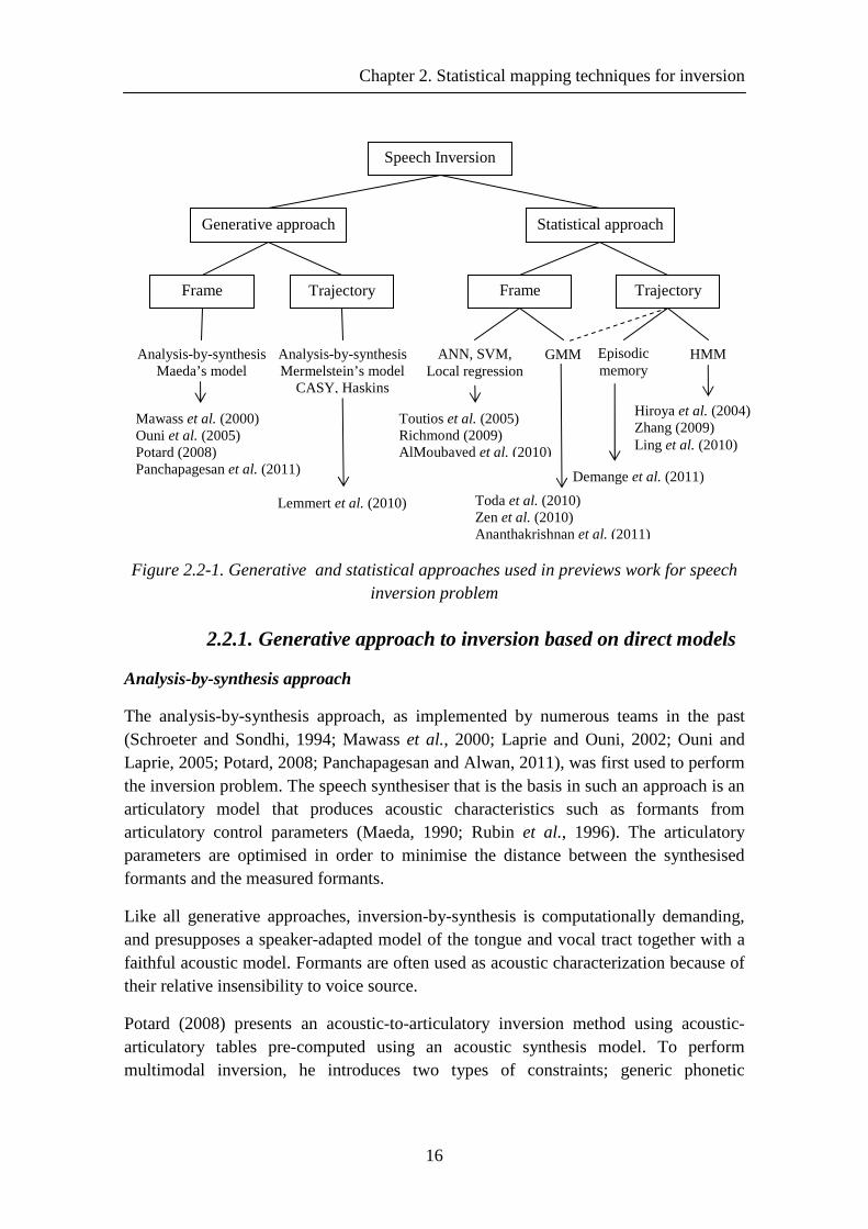
Acoustic-to-articulatory speech inversion mapping problem has been the subject of research for several decades. Because many researchers have been working to perform and improve speech inversion systems for a long time, this section aims to present the major research using physical and statistical approaches. This long-standing problem was testified by the famous work of (Atal et al., 1978). Figure 2.2-1 present a classification of previous work on speech inversion. One approach has been to use articulatory synthesis models, either as part of an analysis-by-synthesis algorithm, or to generate acoustic-articulatory corpora which may be used with a codebook mapping. Much of the more recent works reported have applied machine learning models including HMMs, GMMs or artificial neural networks (ANNs), to human measured articulatory data provided by devices such as the ElectroMagnetic Articulograph (EMA) or marker tracking devices based on classical or infrared video.
Chapter 2. Statistical mapping techniques for inversion
16
Figure 2.2-1. Generative and statistical approaches used in previews work for speech inversion problem
2.2.1. Generative approach to inversion based on direct models
Analysis-by-synthesis approach
The analysis-by-synthesis approach, as implemented by numerous teams in the past (Schroeter and Sondhi, 1994; Mawass et al., 2000; Laprie and Ouni, 2002; Ouni and Laprie, 2005; Potard, 2008; Panchapagesan and Alwan, 2011), was first used to perform the inversion problem. The speech synthesiser that is the basis in such an approach is an articulatory model that produces acoustic characteristics such as formants from articulatory control parameters (Maeda, 1990; Rubin et al., 1996). The articulatory parameters are optimised in order to minimise the distance between the synthesised formants and the measured formants.
Like all generative approaches, inversion-by-synthesis is computationally demanding, and presupposes a speaker-adapted model of the tongue and vocal tract together with a faithful acoustic model. Formants are often used as acoustic characterization because of their relative insensibility to voice source.
Potard (2008) presents an acoustic-to-articulatory inversion method using acoustic-articulatory tables pre-computed using an acoustic synthesis model. To perform multimodal inversion, he introduces two types of constraints; generic phonetic
Hiroya et al. (2004) Zhang (2009) Ling et al. (2010)
Speech Inversion
Generative approach Statistical approach
Frame Trajectory Frame Trajectory
ANN, SVM, Local regression
GMM HMM Episodic memory
Analysis-by-synthesis Mermelstein’s model
CASY, Haskins
Analysis-by-synthesis Maeda’s model
Toutios et al. (2005) Richmond (2009) AlMoubayed et al. (2010)
Demange et al. (2011)
Mawass et al. (2000) Ouni et al. (2005) Potard (2008) Panchapagesan et al. (2011)
Lemmert et al. (2010) Toda et al. (2010) Zen et al. (2010) Ananthakrishnan et al. (2011)
Chapter 2. Statistical mapping techniques for inversion
17
constraints, derived from the analysis by human experts of articulatory invariance for vowels, and visual constraints, derived automatically from the video signal.
Mawass et al (2000) present an articulatory approach to synthesis fricative consonants in vocalic context. The articulatory trajectories of the control parameters for the synthesiser –based on an articulatory model (Beautemps et al., 2001) and a vocal tract electric analog (Badin and Fant, 1984) – are estimated by inversion from audio-video recordings of the reference subject. The articulatory control parameters were determined by an articulatory inversion from formants and lip aperture using a constrained optimisation algorithm based on the gradient descent method. A simple strategy of coordination of the control of the glottis and the oral constriction gesture was used to synthesise voiceless and voiced fricatives. A formal perceptual test based on a forced choice consonant identification demonstrated the high quality of the speech sound. Moreover, the articulatory data obtained by inversion and the methodology developed served as the basis for studying human control strategies for speech production
Panchapagesan and Alwan (2011) presented a quantitative study of acoustic-to-articulatory inversion for vowel speech sounds by analysis-by-synthesis using Maeda’s articulatory model (Maeda, 1988). Using a cost function that includes a distance measure between natural and synthesised first three formants, and parameter regularisation and continuity terms, they calibrate the Maeda model to two speakers, one male and one female, from the University of Wisconsin x-ray micro-beam (XRMB) database. For several vowels and diphthongs for the male speaker, they found smooth articulatory trajectories, an average distances around 0.15 cm, and less than 1% average error in the first three formants between estimated midsagittal vocal tract outlines and measured XRMB tongue pellet positions.
Lammert et al. (2008; 2010) used the CASY articulatory synthesizer (Iskarous et al., 2003) using the Mermelstein articulatory model (Mermelstein, 1973) to train a forward model of the articulatory-to-acoustic transform and its Jacobian using Locally-Weighted Regression (LWR) models and Artificial Neural Networks (ANNs). This functional forward model was however never directly confronted to real data.
Codebook Approach
Also referred to as the articulatory codebooks approach (Schroeter and Sondhi, 1994), the codebook approach builds lookup tables consisting of pairs of segmental acoustic and articulatory parameters from parallel recorded articulatory-acoustic data, or data synthesised by an articulatory synthesiser. (1996) used ElectroMagnetic Articulography (EMA, cf. Chapter 3) data recorded by one Swedish male subject to built a codebook of quantised articulatory-acoustic parameter pairs. In their study, the acoustic vectors created using Vector Quantisation (VQ) were categorised into a lookup table with 256 codes by finding the shortest Euclidean distance between the acoustic vectors and each of a small set of numbered reference vectors. A VQ codebook was used to map from
Chapter 2. Statistical mapping techniques for inversion
18
acoustic segments to VQ codes, and a lookup table was then used to map from the VQ code to an estimated articulatory configuration. (Hogden et al., 1996) reported Root-Mean-Squared (RMS) errors around 2 mm for coils on the tongue. They found that the optimum RMS error over whole test set was produced by a time delay between acoustic and articulatory features of 14.4 ms. The improvement in RMS error due to this delay is about 0.1 mm (i.e. about 5% reduction). Being a discrete method, the VQ approach does not give the same level of approximation to the target distribution without significantly increasing the size of lookup table, compared to methods employing continuous variables. Today this method has largely been replaced by more sophisticated models.
Ouni and Laprie (1999) presents a method to generate a codebook that represents the mapping between articulatory and acoustic domains. Because of the non-linearity between the two domains, the articulatory space is considered as composed of several hypercubes where the mapping is linear. This approach aims to discretize densely the articulatory space only in the regions where the mapping is highly non-linear. For this purpose, a hypercube structure is used. During the mapping process, the information contained in the hypercube structure is used to retrieve the articulatory parameters from the acoustic ones. (Ouni and Laprie, 2005) present the same technique using an adaptive sampling algorithm to ensure that the acoustical resolution is almost independent of the region in the articulatory space. The inversion procedure retrieves articulatory vectors corresponding to acoustic entries from the hypercube codebook. The best articulatory trajectory is estimated using a nonlinear smoothing algorithm together with a regularization technique. The inversion ensures that inverse articulatory parameters generate original formant trajectories with high precision and a realistic sequence of the vocal tract shapes.
The advantage of the physical models is that the implementation does not require experimental data for training, but the method is computationally costly i.e. analysis-by-synthesis approach puts high demands on the quality of the synthesis. In other words, the performance – or counter performance – might result from the synthesis rather than from the inversion. This approach is currently mainly applicable to vowels. In addition, the physical modelling of acoustic and articulatory relationship is complex and difficult to adapt to any new speaker, and the inversion quality depends on the speaker adaptation stage.
2.2.2. Statistical approach to inversion
Another type of approach to acoustic-to-articulatory inversion is based on statistical models of speech production trained on parallel acoustic – articulatory data acquired on real speakers, as can be found in the literature. Globally, we can mention four different classes: Hidden Markov Models (HMMs), Gaussian Mixtures Models (GMMs), Artificial Neural Networks (ANNs), and Support Vector Machines (SVMs). This section describes briefly the methods and results found in the literature (Toda et al.,
Chapter 2. Statistical mapping techniques for inversion
19
2008), (Richmond, 2007), (Toutios and Margaritis, 2005a; Toutios and Margaritis, 2005b), (Zen et al., 2011). In addition to the data, phonetic information can be used: (Hiroya and Honda, 2004), (Zhang and Renals, 2008; Zhang, 2009), (Ling et al., 2010), (Zen et al., 2011).
HMM-based inversion mapping approach
Hiroya and Honda (2004) developed a method that determines the articulatory movements from speech acoustics using an HMM-based speech production model. The corpus used contains 358 sentences (about 18 minutes) spoken at normal rate by three Japanese male subjects. After proper labelling of the recorded corpus, 342 randomly selected sentences were used as training corpus, each allophone is modelled by a context-dependent HMM, and the proper inversion is performed by a state-dependent linear regression between the observed acoustic and the corresponding articulatory parameters. The articulatory parameters of the statistical model are then determined for a given speech spectrum by maximizing a posteriori estimation. In order to assess the importance of phonetics, they tested their method under two experimental conditions, namely with and without phonemic information. In the former, the phone HMMs were assigned according to the correct phoneme sequence for each test utterance. In the latter, the optimal state sequence was determined among all possible state sequences of the phone HMMs and silence model. They found that the average RMS errors of the estimated articulatory parameters were 1.50 mm from the speech acoustics and the phonemic information in the utterance and 1.73 mm from the speech acoustics only.
Zhang and Renals (2008; 2009) developed a similar approach using the MOCHA-TIMIT 1 corpus. Zhang (2009) performs a mean-filtering normalisation to compensate some EMA measure errors introduced in the recording stage (Richmond, 2002) and used the same split of training, validation and test set as used in (Richmond, 2002). He indicates that the jointly trained acoustic-articulatory models are more accurate (having a lower RMS error) than the separately trained ones, and that Trajectory-HMM training results in greater accuracy compared with conventional Baum-Welch parameter updating. Trajectory-HMM training using the Root Mean Square criteria proves to be better than using the standard Maximum Likelihood criteria. The use of triphone models shows that context-dependent is an effective way to improve modelling performance with little added complexity in training. The lowest RMS error of the inversion from speech signal alone was 1.68 mm. Adding the phone labels information to get the states sequence based on forced alignment, the RMS error decrease to 1.4 mm. Zhang and Renals (2008) described a system which jointly optimises multi-stream phone-sized HMMs on synchronous acoustic and articulatory frames. The inversion is carried out in
1 http://www.cstr.ed.ac.uk/research/projects/artic/mocha.html
Chapter 2. Statistical mapping techniques for inversion
20
two stages: first a representative HMM state alignment is derived from the acoustic channel; a smoothed mean trajectory is generated from the HMM state sequence by an articulatory trajectory formation model using the same HMMs. Depending on the availability of the phone labels for the test utterance, the state sequence can be either returned by an HMM decoder, or by forced alignment derived from phone labels, leading to RMS errors of respectively 1.70 mm and 1.58 mm.
Ling et al. (2010) developed a HMM-based prediction of articulatory movements from text, acoustic (inversion) and both text and acoustic input. The male British English speaker recorded 1263 sentences (Richmond, 2009). After automatic labelling of the corpus, they used 1200 sentences to train two forms of context-dependent HMMs (quinphone and fully context-dependent models) in addition to the simple monophone models. For the inversion mapping, monophone and triphone acoustic model was trained and a decision tree-based model clustering was applied to perform the decoding of the triphone model of the acoustic feature to give a phone sequence. They found using quinphone that the average RMS error were 1.94 mm from only text input, 0.90 mm when both text and acoustic features are given as input. Form only acoustic input, phone recognition system was trained using triphone acoustic model. The accuracy of this system was 71.49% and the RMS error was 1.08 mm in this case.
Katsamanis et al.(2009) approximated the audiovisual-to-articulatory mapping by an adaptive piecewise linear model. Model switching was governed by a Markovian discrete process which captures articulatory dynamic information. Each constituent linear mapping is effectively estimated via canonical correlation analysis. For facial analysis, active appearance models demonstrated fully automatic face tracking and visual feature extraction capabilities. Exploiting both audio and visual modalities in a multi-stream HMM-based scheme, they found RMS errors ranging from 0.5 to 2.5 mm, depending on the articulator involved.
GMM-based inversion mapping approach
Toda et al.(2008) described a statistical approach for both articulatory-to-acoustic mapping and acoustic-to-articulatory inversion mapping without phonetic information. Such an approach interestingly enables language-independent speech modification and coding. They modelled the joint probability density of articulatory and acoustic frames in context using GMMs. They employed two different techniques to establish the GMM mappings. They used a 5 fold cross validation procedure based on MOCHA-TIMIT database to evaluate these techniques. Using a minimum mean-square error (MMSE) criterion with an 11 frame acoustic window and 32 mixture components, they obtained RMS inversion errors of 1.61 mm for one female speaker fsew0, and of 1.53 mm for a male speaker mask0. Using maximum likelihood estimation (MLE) method and 64 mixture components, they improved their results to 1.45 mm for fsew0, and 1.36 mm for mask0. Note that in order to improve the mapping performance, they smoothed the
Chapter 2. Statistical mapping techniques for inversion
21
estimated articulatory trajectories by lowpass filtering (e.g., Richmond, 2002). In addition, the optimum cutoff frequency of the lowpass filter was determined to minimise the minimum RMS error of the test data in each dimension of the articulatory vector.
Zen et al. (2010) propose a technique of continuous stochastic feature mapping based on trajectory HMM compared to the trajectory GMM. Although GMM or HMM feature mapping techniques work successfully, the trajectories are sometimes discontinuous because of frame-to-frame mapping. To alleviate this problem, they used the dynamic feature constrains at the mapping stage. This constrains also introduces inconsistencies between training and mapping. The proposed technique can eliminate these inconsistencies and offer entire sequence-level transformation rather than frame-to-frame mapping. Using the same normalisation technique for the measured EMA and also the same training, validation and test partition as in (Richmond, 2002), they found an average RMS error of 1.52 mm for trajectory HMM using the correct transcription for the msak0 speaker of MOCHA-TIMIT corpus. On the other hand, the average RMS error was 1.13 mm for trajectory GMMs. Note that they tested this techniques on other task i.e. speaker conversion and noise compensation and found better performance for the trajectory HMM/GMM than standard ones.
Ananthakrishnan and Engwall (2011) propose a definition for acoustic and articulatory gestures using a method that segments the measured articulatory trajectories and acoustic waveforms into gestures. Using a simultaneously recorded acoustic-articulatory database, they used critical points in the utterance to detect the gestures for both acoustic and articulatory representations. They studied the relationship between the detected acoustic and articulatory gestures in terms of the timing as well as the shape. In order to study this relationship further, they perform an acoustic-to-articulatory inversion using GMM-based regression. Using the two speakers of the MOCHA-TIMIT corpus, they performed 10-fold cross-validation and normalised the MFCC and the articulatory trajectory vectors of the training data to zero mean with a Standard Deviation (SD) of 1. They found an average error of 1.45 mm and 1.55 mm for the male and the female speakers, respectively. In order to evaluate the acoustic-to-articulatory inversion in a more intuitive manner, they suggested a method based on the error at the estimated critical points. Using this method, they noted that the estimated articulatory trajectories using the acoustic-to-articulatory inversion methods were still not accurate enough to be within the perceptual tolerance of audio-visual asynchrony.
Neural network-based inversion mapping approach
Richmond (2002) used fsew0 of MOCHA-TIMIT corpus as training, validation and testing data. He used the files whose numbers end with 2 for validation (46 utterances), those ending with 6 for testing (46 utterances) and the remaining 368 utterances for training. To compensate some EMA measure errors introduced in the recording stage,
Chapter 2. Statistical mapping techniques for inversion
22
Richmond (2002) performed a mean-filtering normalisation. He used the mixture density network (MDN). In the most general sense, the MDN can be considered as combining a trainable regression function (typically a non-linear regressor such as an artificial neural network) with a probability density function. A multilayer perceptron (MLP) was used as a trainable non-linear regressor and a GMM. The role of the MLP is to take an input vector in acoustic domain and map to the articulatory domain. Training consists of updating the MLP weights to optimize an error function, defined as the negative log likelihood of the target data. Thus, standard nonlinear optimization algorithms may be used to train the MDN. Since, the MDN gives a model of conditional probability density, it is trivial to augment the target features with derived delta and delta-delta features i.e. dynamic features. Once trained, the input sequence of acoustic feature vectors gets an output of a sequence of pdfs over the static and dynamic articulatory features. The maximum likelihood parameter generation algorithm (MLPG) (Tokuda et al., 2000) was applied to this sequence of pdfs in order to obtain a single, most probable trajectory which optimizes the constraints between the static and dynamic features. In the case of a sequence of pdfs containing a single Gaussian mixture component, the optimum is the solution of a set of linear equations. When multiple mixture components are used, an EM-based algorithm is applied. The MLP output trajectories were lowpass filtered using cutoff frequencies derived empirically by lowpass filtering the validation data set. The average RMS error values using MLP with 38 hidden units was 1.62 mm for the unfiltered output and decreased to an average of 1.57 mm for the filtered one. The average RMS error for the tongue coils was 2.2 mm. Richmond et al. (2003) also modelled the mapping using a neural network based on mixture density estimation. It has been reported that the multiple representation of articulatory probability density is effective for the inversion mapping. More recently, the trajectory mixture density network (TMDN) approach with many more free parameters has resulted in a decreased RMS error to 1.40 mm on the same training, validation and testing datasets (Richmond, 2007). (Richmond, 2009) apply TMDN to a new corpus of articulatory data. This new data set, mngu0, is relatively large and phonetically rich, among other beneficial characteristics. Three subsets were created from a total set of 1,263 recorded utterances: a training set of 1,137 utterances; a validation set of 63 utterances comprising; and a test set with the remaining 63 utterances. The obtained result was good, with an RMS error of 0.99 mm. This compares very well with the previous lowest result RMS error for equivalent coils of the MOCHA fsew0 EMA data. The interpretation of this confirms that the statistical method for inversion is very much related to the corpus.
Qin and Carreira-Perpiñán (2007) study empirically the best acoustic parameterisation for articulatory inversion. They compare all combinations of the following factors: 1) popular acoustic features such as MFCC and PLP with and without dynamic features; 2) time delay effect; 3) different levels of smoothing of the acoustic temporal trajectories. Using multilayer perceptron (MLP) to map from acoustic features to articulatory ones,
Chapter 2. Statistical mapping techniques for inversion
23
experimental results on a real speech production database show consistent improvement when using features closely related to the vocal tract (in particular LSF), dynamic features, and large window length and smoothing (which reduce the jaggedness of the acoustic trajectory). Further improvements are obtained with a 15 ms time delay between acoustic and articulatory frames. However, the improvement attained over other combinations is very small (at most 0.3 mm RMS error) compared to a minimum RMS error of around 1.65 mm.
Kjellström and Engwall (2009) implemented an audiovisual-to-articulatory inversion using simple multi-linear regression or ANNs. Depending on the type of fusion (early or late) between the audio signal and the video signal (based on independent component images of the mouth region), they obtained RMS reconstruction errors for the tongue shape ranging from 2.5 to 3 mm.
Support vector regression-based inversion mapping approach
Toutios and Margaritis (2005a; 2005b) employ the machine learning technique of Support Vector Regression (SVR) (Smola and Schölkopf, 2004) on speech inversion. They used the same data set as Richmond (2002). Because the SVR works for only one output, they split the inversion problem in 14 distinct functions considering each time a different EMA coordinate trajectory as output. Using principal analysis component (PCA), they move to a new output space of all 14 principal components. PCA lead to only a slight decrease of the RMS error and they found an average RMS error of 1.66 mm.
Local regression-based inversion mapping approach
Al Moubayed and Ananthakrishnan (2010) developed an acoustic-to-articulatory inversion system using local regression on the MOCHA-TIMIT corpus. They discussed two methods of local regression and found that the local non-parametric regression has an optimum performance with 1.56 mm of RMSE, while the local linear regression has an optimum performance of 1.52 mm of RMSE. A maximum likelihood trajectory smoothing using the estimated dynamics of the articulators has a higher effect on local linear regression as compared to local non-parametric regression. Using the same acoustic and articulatory features, they found that the local linear regression is significantly better than the regression using Gaussian Mixture Models.
Episodic memory-based inversion mapping approach
Demange and Ouni (2011) proposed an acoustic-to-articulatory inversion method based on the episodic memory. This method does not rely on any assumptions about the mapping function but rather relies on real synchronised acoustic and articulatory data streams. The memory structurally embeds the naturalness of the articulatory dynamics. In addition, they introduce the concept of generative episodic memory, which enables the production of unseen articulatory trajectories according to the acoustic signals to be
Chapter 2. Statistical mapping techniques for inversion
24
inverted. They used the MOCHA corpus with the same utterances selected for training, development and test sets as in Richmond (2002). Without using any phonemic knowledge they found an average RMSE of 1.63 mm and 1.68 mm for the male and the female speaker, respectively. Using the phonemic segmentation of the test records the average RMS error decreases to 1.45 mm and 1.54 mm for the male and the female, respectively.
2.2.3. Discussion
The acoustic-to-articulatory mapping is a difficult problem because of the one-to-many mapping between the acoustic and articulatory features; one acoustic vector can be produced by more than one articulatory configuration. This chapter presents several studies of inversion task using different approaches. The goal of all the studies described above is to recover the articulators’ movement and to reduce the impact of non-uniqueness as perfectly as possible at all time. It is however difficult to confront the performance of the proposed solutions since metrics, data, speakers and languages are not comparable. The corpora as well as training and testing conditions are also not completely comparable. Note also that the global accuracy of the inversion (i.e. RMSE) was measured in different ways (cf. Section 4.2.2, equation (4.2-2) and (4.2-3)). We however provide a comparison of our results with those of the literature described above in Table 4.5-1.
There is no doubt that the most popular choice of acoustic modelling for both speech recognition and synthesis is the HMM. This technique was successfully applied for speech inversion. The GMM-based technique was also successfully applied for speech inversion mapping. The main difference between HMM-based and GMM-based mappings is that HMMs use phonetic representation as an intermediate between acoustic and articulatory features. On the other side, GMMs map directly the acoustic features with the articulatory ones without the use of any other information. In order to compare the impact of phonetic information, we choose to use HMM and GMM based mapping to develop and to evaluate two inversion systems.
In the next sections, we present the two statistical techniques that we have used: the HMM-based inversion mapping method based on phonetic information and the GMM-based mapping based on direct acoustic-to-articulatory frames mapping without any phonetic information i.e. inversion at frame level.
2.3. HMM-based speech recognition and synthesis
As mentioned above, Hidden Markov Models (HMMs) have become more popular in the development of speech inversion systems. During the past several years, they have successfully been applied to modelling sequences of speech spectra in Automatic Speech recognition (ASR) and Text To Speech synthesis (TTS), and their performance have been improved by several techniques.
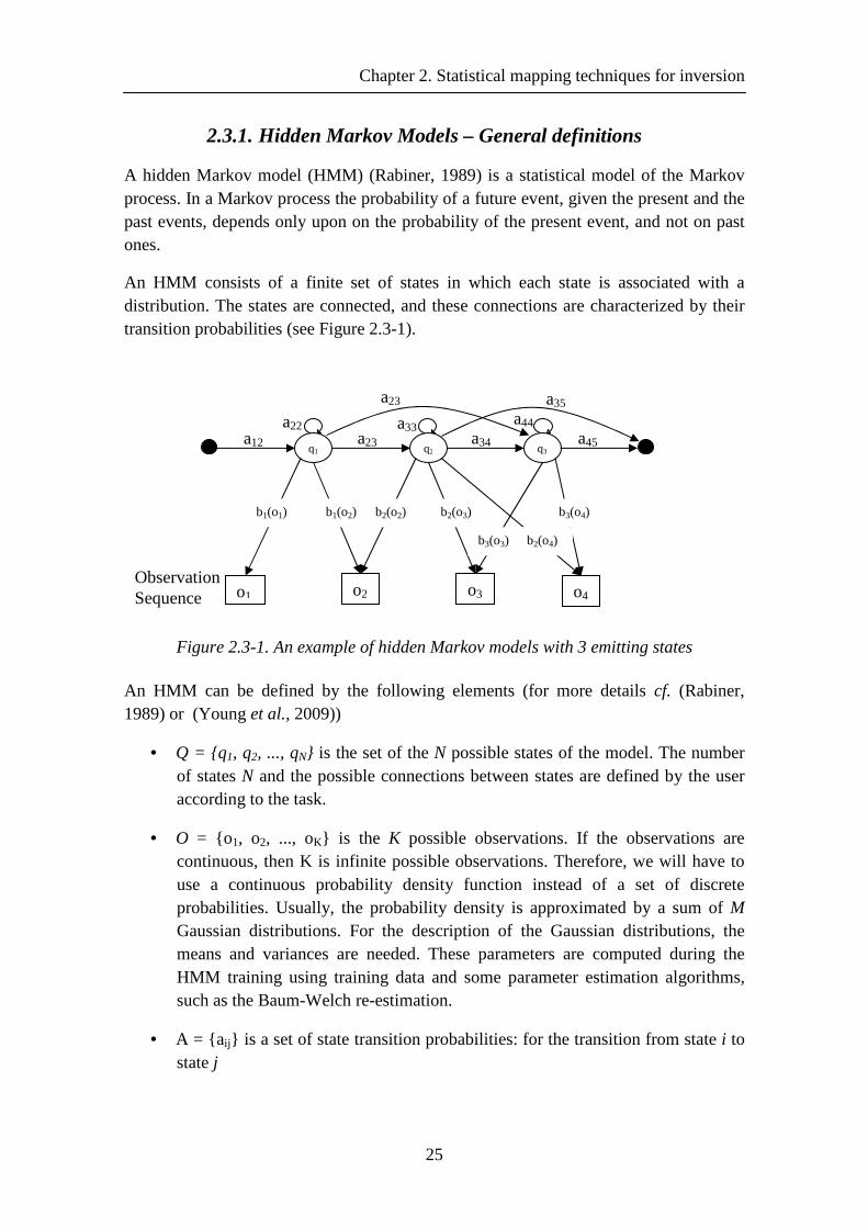
Chapter 2. Statistical mapping techniques for inversion
25
2.3.1. Hidden Markov Models – General definitions
A hidden Markov model (HMM) (Rabiner, 1989) is a statistical model of the Markov process. In a Markov process the probability of a future event, given the present and the past events, depends only upon on the probability of the present event, and not on past ones.
An HMM consists of a finite set of states in which each state is associated with a distribution. The states are connected, and these connections are characterized by their transition probabilities (see Figure 2.3-1).
Figure 2.3-1. An example of hidden Markov models with 3 emitting states
An HMM can be defined by the following elements (for more details cf. (Rabiner, 1989) or (Young et al., 2009))
• Q = {q1, q2, ..., qN} is the set of the N possible states of the model. The number of states N and the possible connections between states are defined by the user according to the task.
• O = {o1, o2, ..., oK} is the K possible observations. If the observations are continuous, then K is infinite possible observations. Therefore, we will have to use a continuous probability density function instead of a set of discrete probabilities. Usually, the probability density is approximated by a sum of M Gaussian distributions. For the description of the Gaussian distributions, the means and variances are needed. These parameters are computed during the HMM training using training data and some parameter estimation algorithms, such as the Baum-Welch re-estimation.
• A = {aij} is a set of state transition probabilities: for the transition from state i to state j
q1 q2 q3
o1 o2 o3
a22
a23
a23
a35
a34 a45 a12
a33 a44
o4
b1(o2) b1(o1) b2(o2) b3(o4)
b2(o4)
b2(o3)
b3(o3)
Observation Sequence
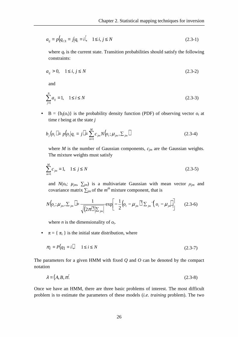
Chapter 2. Statistical mapping techniques for inversion
26
( ) Njiiqjqpa ttij ≤≤=== + ,1,1 (2.3-1)
where qt is the current state. Transition probabilities should satisfy the following constraints:
Njiaij ≤≤> ,1,0 (2.3-2)
and
NiaN
jij ≤≤=∑
=
1,11
(2.3-3)
• B = {bj(ot)} is the probability density function (PDF) of observing vector ot at time t being at the state j
( ) ( ) ( )∑=
∑===M
mjmjmtjmtttj oNcjqopob
1
,; µ (2.3-4)
where M is the number of Gaussian components, cjm are the Gaussian weights. The mixture weights must satisfy
NjcM
mjm ≤≤=∑
=
1,11
(2.3-5)
and N(ot; µjm, ∑jm) is a multivariate Gaussian with mean vector µjm and covariance matrix ∑jm of the mth
mixture component, that is
( )( )
( ) ( )
−∑−−∑
=∑−Τ
jmtjmjmt
jmnjmjmt oooN µµ
πµ 1
2
1exp
2
1,; (2.3-6)
where n is the dimensionality of ot.
• π = { πi } is the initial state distribution, where
( ) NiiqPi ≤≤== 1,1π (2.3-7)
The parameters for a given HMM with fixed Q and O can be denoted by the compact notation
( )πλ ,,BA= (2.3-8)
Once we have an HMM, there are three basic problems of interest. The most difficult problem is to estimate the parameters of these models (i.e. training problem). The two
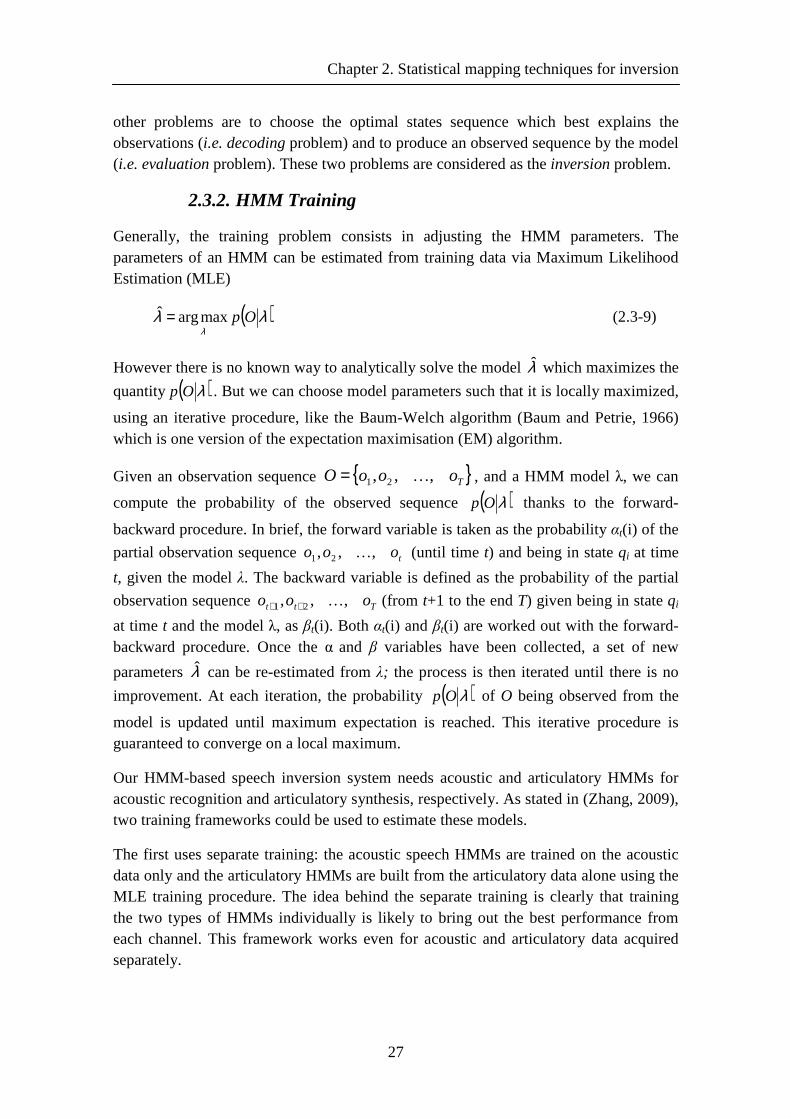
Chapter 2. Statistical mapping techniques for inversion
27
other problems are to choose the optimal states sequence which best explains the observations (i.e. decoding problem) and to produce an observed sequence by the model (i.e. evaluation problem). These two problems are considered as the inversion problem.
2.3.2. HMM Training
Generally, the training problem consists in adjusting the HMM parameters. The parameters of an HMM can be estimated from training data via Maximum Likelihood Estimation (MLE)
( )λλλ
Opmaxargˆ = (2.3-9)
However there is no known way to analytically solve the model λ̂ which maximizes the
quantity ( )λOp . But we can choose model parameters such that it is locally maximized,
using an iterative procedure, like the Baum-Welch algorithm (Baum and Petrie, 1966) which is one version of the expectation maximisation (EM) algorithm.
Given an observation sequence { }ToooO ,,, 21 K= , and a HMM model λ, we can
compute the probability of the observed sequence ( )λOp thanks to the forward-
backward procedure. In brief, the forward variable is taken as the probability αt(i) of the
partial observation sequence tooo ,,, 21 K (until time t) and being in state qi at time
t, given the model λ. The backward variable is defined as the probability of the partial
observation sequence Ttt ooo ,,, 21 K++ (from t+1 to the end T) given being in state qi
at time t and the model λ, as βt(i). Both αt(i) and βt(i) are worked out with the forward-backward procedure. Once the α and β variables have been collected, a set of new
parameters λ̂ can be re-estimated from λ; the process is then iterated until there is no
improvement. At each iteration, the probability ( )λOp of O being observed from the
model is updated until maximum expectation is reached. This iterative procedure is guaranteed to converge on a local maximum.
Our HMM-based speech inversion system needs acoustic and articulatory HMMs for acoustic recognition and articulatory synthesis, respectively. As stated in (Zhang, 2009), two training frameworks could be used to estimate these models.
The first uses separate training: the acoustic speech HMMs are trained on the acoustic data only and the articulatory HMMs are built from the articulatory data alone using the MLE training procedure. The idea behind the separate training is clearly that training the two types of HMMs individually is likely to bring out the best performance from each channel. This framework works even for acoustic and articulatory data acquired separately.
Chapter 2. Statistical mapping techniques for inversion
28
The second scheme, on the other hand, aims to jointly optimise a single model for both acoustic and articulatory information. The model therefore has acoustic and articulatory components, both modelled as multi-state phone-level HMMs: (1) acoustic HMMs that perform an acoustic recognition stage that produces a string of phones and the associated state durations, and (2) articulatory HMMs which generate articulatory trajectories from this string of phones with their durations. Both the acoustic and articulatory models have the same topology, i.e. they have exactly the same set of HMM states and allophonic variations. This structure enables to establishe a stronger bridge between the acoustic and articulatory speech domains and the same phone boundaries for both acoustic and articulatory streams.
Note that the first training framework has to explicitly cope with AV asynchrony if any: there is no guaranty that the best alignment of phone-sized acoustic models directly corresponds to the optimal chaining of phone-sized articulatory models. One solution consists in learning a phasing model such as proposed by Govokhina et al. (2007) for audiovisual speech synthesis or by Saino et al (2006) for computing time-lags between notes of the musical score and sung phones for an HMM-based singing voice synthesis system. The second scheme on the contrary preserves inter-stream asynchrony because internal states of each stream learn static and dynamic characteristics of each corresponding parameters. Transient states are therefore not forced to be captured by the same states: asynchronies are here just of consequence of statistical learning in a way similar to the triphone model for tongue kinematics early proposed by Okadome et al. (1999).
As expected, Zhang (2009) found that training jointly the acoustic and articulatory features in a multi-stream HMM leads to more accurate inversion results than training them separately.
The phone-sized HMM are modelled by joint probability densities of acoustic and articulatory parameters. These models can be enriched in many ways:
• Use of dynamic (delta) features. (Furui, 1986; Masuko et al., 1996). Dynamic features, i.e. first time derivative of the features, can be exploited by trajectories HMMs to smooth trajectories.
• Context-dependent HMMs. Due to coarticulatory effects, it is unlikely that a single context-independent HMM could optimally represent a given allophone. Therefore context-dependent HMMs are used as another way to enrich the model. The idea of context-dependent modelling is that, instead of defining phones, we define phones in their contexts. We define a left context with a minus "-" sign, and a right context with a plus "+" sign. For example, the phone "i" bounded by a "b" and a "p" is now modelled by: “b-i+p”. Because of the limited training data available for our system, we use context classes of phonemes as contexts, in order to have more occurrences for each class and to
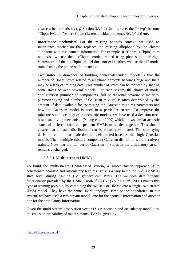
Chapter 2. Statistical mapping techniques for inversion
29
ensure a better statistics (cf. Section 3.3.1.2). In this case, the “b-i+p” become “Cbpm-i+Cbpm” where Cbpm clusters bilabial phonemes /b/, /p/ and /m/.
• Inheritance mechanism. For the missing phone’s context, we used an inheritance mechanism that replaces the missing allophone by the closest allophone with less context information. For example, if “Cbpm-i+Cbpm” does not exist, we use the “i+Cbpm” model trained using phones in their right context, and if the “i+Cbpm” model does not exist either, we use the “i” model trained using the phone without context.
• Tied states. A drawback of building context-dependent models is that the number of HMM states related to all phone contexts becomes huge and there may be a lack of training data. This number of states can be reduced by sharing some states between several models. For each stream, the choice of model configuration (number of components, full or diagonal covariance matrices, parameter tying and number of Gaussian mixture) is often determined by the amount of data available for estimating the Gaussian mixtures parameters and how the Gaussian model is used in a particular stream. To improve the robustness and accuracy of the acoustic models, we have used a decision tree–based state tying mechanism (Young et al., 2009) which allows similar acoustic states of different context-dependent HMMs to be tied together. This should ensure that all state distributions can be robustly estimated. The state tying decision tree in the acoustic domain is elaborated based on the single Gaussian models. Then, multiple mixture component Gaussian distributions are iteratively trained. Note that the number of Gaussian mixtures in the articulatory stream remains unchanged.
2.3.2.1 Multi-stream HMMs
To build the multi-stream HMM-based system, a simple fusion approach is to concatenate acoustic and articulatory features. This is a way to tie the two HMMs at state level during training (i.e. synchronous state). The multiple data streams functionality provided by the HMM ToolKit2 (HTK) (Young et al., 2009) makes this type of training possible, by combining the two sets of HMMs into a single, two-stream HMM model. They have the same HMM topology, same phone boundaries. In our system, we have used a two-stream model: one for the acoustic information and another one for the articulatory information.
Given the multi-stream observation vector O, i.e. acoustic and articulatory modalities, the emission probability of multi-streams HMM is given by
2 http://htk.eng.cam.ac.uk/
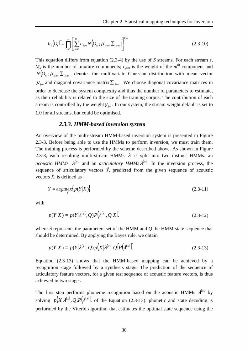
Chapter 2. Statistical mapping techniques for inversion
30
( ) ( )∏ ∑= =
∑=
S
s
M
mjsmjsmstjsmtj
jsts
ONcOb1 1
,;γ
µ (2.3-10)
This equation differs from equation (2.3-4) by the use of S streams. For each stream s, Ms is the number of mixture components; cjsm is the weight of the mth component and
( )jsmjsmstON ∑,;µ denotes the multivariate Gaussian distribution with mean vector
jsmµ and diagonal covariance matrixjsm∑ . We choose diagonal covariance matrices in
order to decrease the system complexity and thus the number of parameters to estimate, as their reliability is related to the size of the training corpus. The contribution of each
stream is controlled by the weightjstγ . In our system, the stream weight default is set to
1.0 for all streams, but could be optimised.
2.3.3. HMM-based inversion system
An overview of the multi-stream HMM-based inversion system is presented in Figure 2.3-3. Before being able to use the HMMs to perform inversion, we must train them. The training process is performed by the scheme described above. As shown in Figure 2.3-3, each resulting multi-stream HMMs λ is split into two distinct HMMs: an
acoustic HMMs ( )xλ and an articulatory HMMs ( )yλ . In the inversion process, the sequence of articulatory vectors Ŷ, predicted from the given sequence of acoustic vectors X, is defined as
{ })(maxargˆ XYpYY
= (2.3-11)
with
( ) ( )( )XQPQYpXYp xy ,),()( λλ= (2.3-12)
where λ represents the parameters set of the HMM and Q the HMM state sequence that should be determined. By applying the Bayes rule, we obtain
( ) ( )( ) ( )( )xxy PQXpQYpXYp λλλ ,),()( = (2.3-13)
Equation (2.3-13) shows that the HMM-based mapping can be achieved by a recognition stage followed by a synthesis stage. The prediction of the sequence of articulatory feature vectors, for a given test sequence of acoustic feature vectors, is thus achieved in two stages.
The first step performs phoneme recognition based on the acoustic HMMs ( )xλ by
solving ( )( ) ( )( )xx PQXp λλ , of the Equation (2.3-13): phonetic and state decoding is
performed by the Viterbi algorithm that estimates the optimal state sequence using the
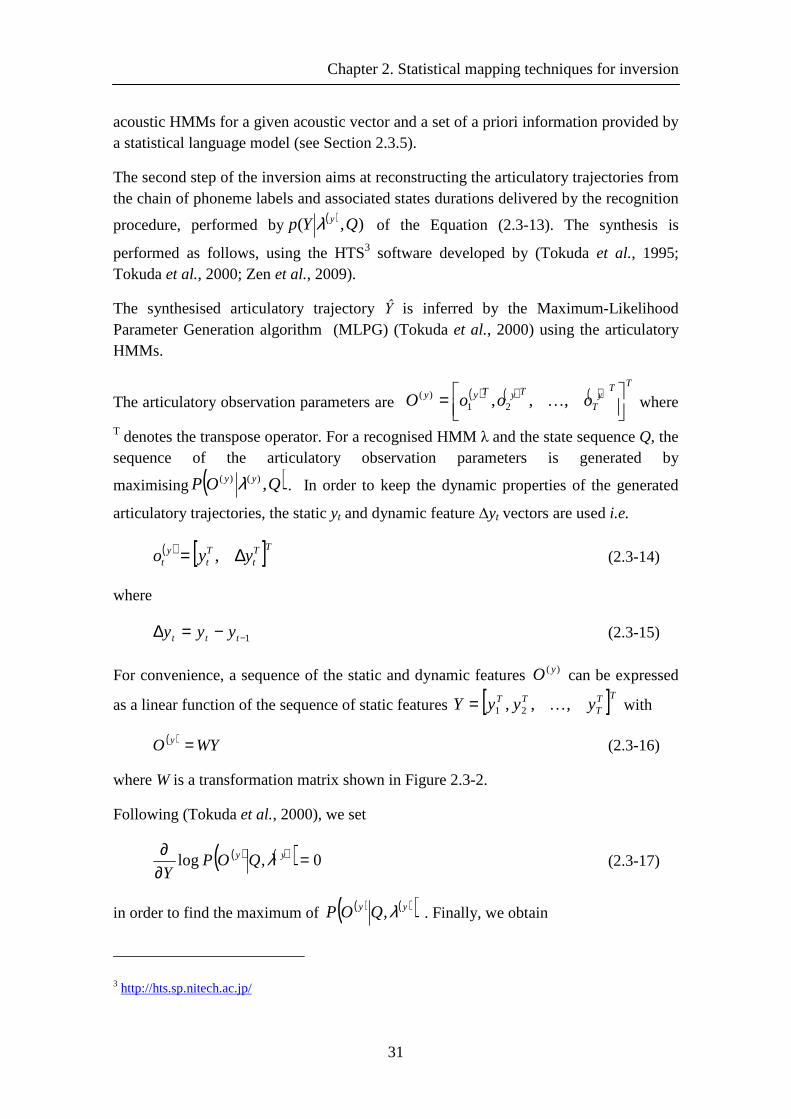
Chapter 2. Statistical mapping techniques for inversion
31
acoustic HMMs for a given acoustic vector and a set of a priori information provided by a statistical language model (see Section 2.3.5).
The second step of the inversion aims at reconstructing the articulatory trajectories from the chain of phoneme labels and associated states durations delivered by the recognition
procedure, performed by ( ) ),( QYp yλ of the Equation (2.3-13). The synthesis is
performed as follows, using the HTS3 software developed by (Tokuda et al., 1995; Tokuda et al., 2000; Zen et al., 2009).
The synthesised articulatory trajectory Ŷ is inferred by the Maximum-Likelihood Parameter Generation algorithm (MLPG) (Tokuda et al., 2000) using the articulatory HMMs.
The articulatory observation parameters are ( ) ( ) ( )
TTy
T
TyTyy oooO
= ,,, 21
)(K where
T denotes the transpose operator. For a recognised HMM λ and the state sequence Q, the sequence of the articulatory observation parameters is generated by
maximising ( )QOP yy ,)()( λ . In order to keep the dynamic properties of the generated
articulatory trajectories, the static yt and dynamic feature ∆yt vectors are used i.e.
( ) [ ]TTt
Tt
yt yyo ∆= , (2.3-14)
where
1−−=∆ ttt yyy (2.3-15)
For convenience, a sequence of the static and dynamic features )( yO can be expressed
as a linear function of the sequence of static features [ ]TTT
TT yyyY ,,, 21 K= with
( ) WYO y = (2.3-16)
where W is a transformation matrix shown in Figure 2.3-2.
Following (Tokuda et al., 2000), we set
( ) ( )( ) 0,log =∂∂ yy QOPY
λ (2.3-17)
in order to find the maximum of ( ) ( )( )yy QOP λ, . Finally, we obtain
3 http://hts.sp.nitech.ac.jp/
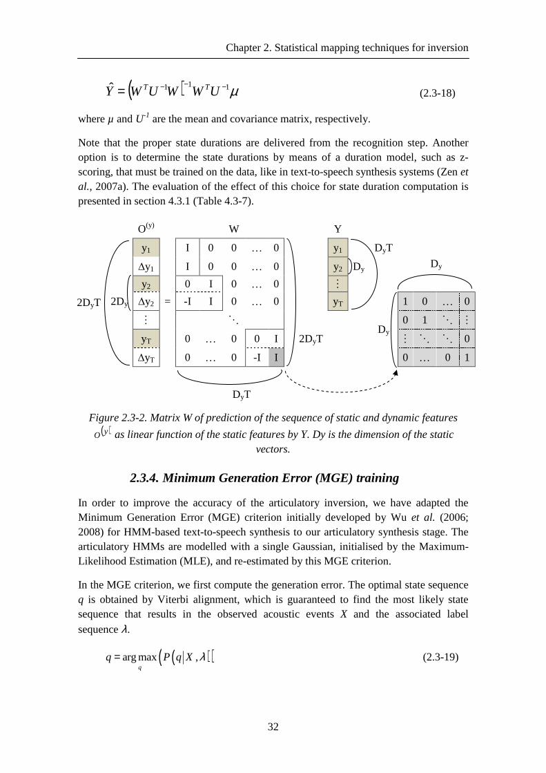
Chapter 2. Statistical mapping techniques for inversion
32
( ) µ111ˆ −−−= UWWUWY TT
(2.3-18)
where µ and U-1 are the mean and covariance matrix, respectively.
Note that the proper state durations are delivered from the recognition step. Another option is to determine the state durations by means of a duration model, such as z-scoring, that must be trained on the data, like in text-to-speech synthesis systems (Zen et al., 2007a). The evaluation of the effect of this choice for state duration computation is presented in section 4.3.1 (Table 4.3-7).
Figure 2.3-2. Matrix W of prediction of the sequence of static and dynamic features ( )yO as linear function of the static features by Y. Dy is the dimension of the static
vectors.
2.3.4. Minimum Generation Error (MGE) training
In order to improve the accuracy of the articulatory inversion, we have adapted the Minimum Generation Error (MGE) criterion initially developed by Wu et al. (2006; 2008) for HMM-based text-to-speech synthesis to our articulatory synthesis stage. The articulatory HMMs are modelled with a single Gaussian, initialised by the Maximum-Likelihood Estimation (MLE), and re-estimated by this MGE criterion.
In the MGE criterion, we first compute the generation error. The optimal state sequence q is obtained by Viterbi alignment, which is guaranteed to find the most likely state sequence that results in the observed acoustic events X and the associated label sequence λ.
( )( )arg max ,q
q P q X λ= (2.3-19)
O(y) W Y
2DyT
y1 I 0 0 L 0
y1 DyT
∆y1 I 0 0 L 0 y2 Dy Dy
y2 0 I 0 L 0 M
2Dy ∆y2 = -I I 0 L 0 yT
Dy
1 0 L 0
M O 0 1 O M yT 0 L 0 0 I 2DyT M O O 0
∆yT 0 L 0 -I I 0 L 0 1
DyT
Chapter 2. Statistical mapping techniques for inversion
33
For a given state sequence q, the generation error ( )YYD ˆ, is defined by the Euclidean
distance between the generated articulatory trajectories Ŷ using Equation (2.3-18) and measured trajectories Y, i.e.
( ) ∑=
=−=T
ttt yyYYYYD
1
22ˆ,ˆˆ, (2.3-20)
The Generalized Probabilistic Descent (GPD) algorithm (Blum, 1954) is used in the
parameter updating stage with the aim to minimize ( )YYD ˆ, over the training set, and is
implemented as:
( )
∑= =∂
−∂−=N
n
nnold
old
yyD
1update
ˆ
λλλελλ
(2.3-21)
where N is the total number of the training sample related to λ and 1
2Nε = is the step
size where N is the total frames related to current updated model. From Equation (2.3-18) and Equation (2.3-20), the updating rule for the mean parameter µ can be formatted as
( ) ( )
µε
µ ∂∂−=
∂−∂ Y
YYYYD T ˆ
ˆ2ˆ
(2.3-22)
where
( ) µµZUWWUW
Y TT 111ˆ
−−−=∂∂
(2.3-23)
Finally,
( ) ( ) µεµµ ZUWWUWYY TTT
nnold111
updateˆ2 −−−−−=
(2.3-24)
Considering that WWT is a quasi diagonal matrix and diagonal elements are larger than other elements, we made an approximation as WWT ≈ a I where I is an unit matrix and a is a constant number for normalization. We apply this approximation to the mean vector by using a = 1, which leads to:
( ) µεµµ ZWYY TT
nnold −−= ˆ2update (2.3-25)
( )origgenold µµµ −−=
(2.3-26)
Chapter 2. Statistical mapping techniques for inversion
34
The simplified updating rules of the HMM parameter is detailed in (Wu et al., 2006) Similarly, the covariance parameter υ=1/σ2 corresponding to µ can be updated as
( ) ( ) ( )YWZWWUWYY TTT
nnoldˆˆ2
11update −−−= −− µευυ υ
(2.3-27)
( )( )∑∑= =
−−−=N
n
T
ttntntntn ooo
1 1,,,,
2old
2update ˆˆ2 µεσσ
(2.3-28)
When we used the above simplification to the Equation (2.3-18), we found
( ) µµ TTT WUWWUWY ≈= −−− 111ˆ (2.3-29)
This Equation (2.3-29) was used in the updating rules. We can see the parameter of the synthesised frame is generated by using the static and dynamic feature of the related state.
We have implemented this algorithm by coupling the HERest procedure from the HTK toolkit and the HMGenS procedure from HTS. The HERest procedure is the core of HTK training toolbox (Young et al., 2009). It implements the forward and backward passes for the re-estimation of the whole set of HMM phone models simultaneously. The HMGenS procedure is a speech parameter generation tool based on the expectation-maximization (EM) algorithm (Zen et al., 2007b).
2.3.5. Language models
In order to improve the recognition performance, a stochastic language model can be used to help constrain the selection to a linguistically meaningful state sequence. This takes into account that all phone sequences are not necessarily equally likely. The language model gives the probability of observing a particular phone sequence. As shown in Equation (2.3-13), the language model has a significant effect on the intermediate recognition accuracy, but the consequence on the final estimation is not straightforward.
To estimate P(λ), a phone transcription of a text corpus that contain phonetic transcriptions (i.e. many phone sequences) is used. P(λ) can be estimated for an N-gram language model by
( ) ( ) ( )1 21
, ,...,Tp
N i i i i Ni
P P Pλ λ λ λ λ λ− − −=
= = ∏ (2.3-30)
where λi is the i th phone and Tp is the total number of phones.
The choice of a language model will depend on the application. We have tested two models: (1) a simple phonotactic grammar can be used to indicate that phonemes in
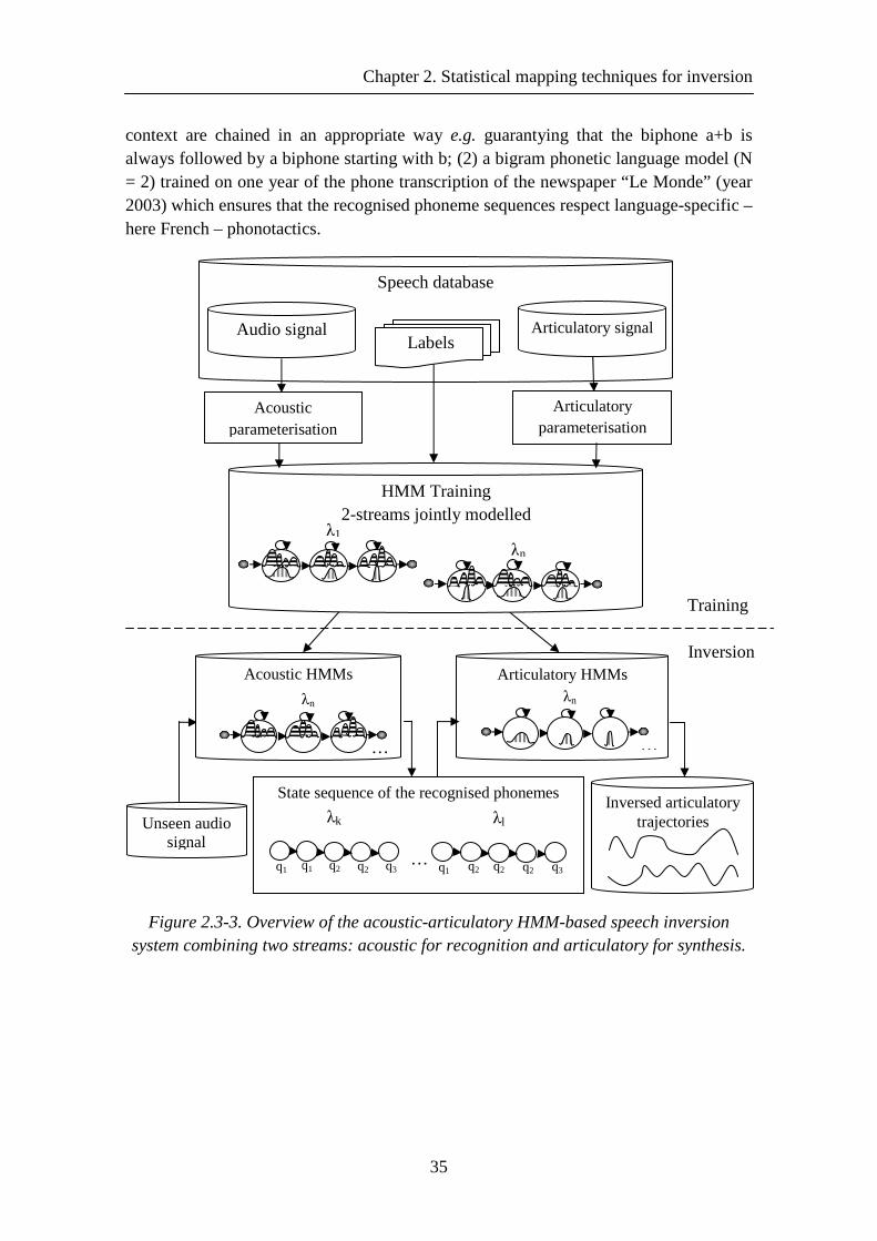
Chapter 2. Statistical mapping techniques for inversion
35
context are chained in an appropriate way e.g. guarantying that the biphone a+b is always followed by a biphone starting with b; (2) a bigram phonetic language model (N = 2) trained on one year of the phone transcription of the newspaper “Le Monde” (year 2003) which ensures that the recognised phoneme sequences respect language-specific – here French – phonotactics.
Figure 2.3-3. Overview of the acoustic-articulatory HMM-based speech inversion system combining two streams: acoustic for recognition and articulatory for synthesis.
Articulatory parameterisation
Articulatory HMMs
Inversed articulatory trajectories
State sequence of the recognised phonemes
q2 q2 q1 q1
λk
q3 … q2 q2 q2 q1
λl
q3
Inversion
Unseen audio signal
…
… λn
Acoustic HMMs
…
λn …
Training
Speech database
Articulatory signal Audio signal Labels
HMM Training 2-streams jointly modelled
…
…
λ1 λn
Acoustic parameterisation
Chapter 2. Statistical mapping techniques for inversion
36
2.4. GMM-based direct inversion
The Gaussian Mixture Models (GMMs) constitute another class of statistical models. GMMs are used as a statistical model of the probability distribution of continuous measurements (i.e. features).
The GMM-based mapping is often used for voice conversion (Stylianou et al., 1998), (Toda and Shikano, 2005), (Tran, 2010) and in both articulatory-to-acoustic and acoustic-to-articulatory mapping (Toda et al., 2004a; Toda et al., 2008). It predicts directly the articulatory features from the acoustic features without passing through a symbolic representation as with the HMMs. In order to compare the performance of the recognition and synthesis HMM-based inversion approach with this direct GMM mapping approach, we implemented a GMM-based acoustic-to-articulatory speech inversion system.
2.4.1. Gaussian Mixture Models – General definitions
Gaussian Mixture Models (GMMs) are among the most statistically mature methods for clustering. Though, they are also used intensively for density estimation. A GMM is a parametric probability density function represented as a weighted sum of Gaussian component densities. GMMs are usually used as a parametric model of the probability distribution of continuous measurements. GMM parameters are estimated from training data using, for example, the iterative Expectation-Maximisation (EM) algorithm.
The complete Gaussian mixture model is parameterised by the mean vectors µ, covariance matrices ∑ and mixture weights w from all component densities. These parameters are collectively represented by the notation:
( )∑= ,,µλ w (2.4-1)
The next section describes the training procedure used to estimate these parameters.
Notice that the states of unsupervised HMM that can take into account the temporal dimension of speech to preserve the continuity is similar to the GMM, which does not need any phonetic information (i.e. phoneme segmentation and labelling) (Lachambre et al., 2011).
2.4.2. GMM Training based on EM algorithm
As for the HMMs, the GMMs parameters must be estimated in a training phase before the GMMs can be used for inversion. In this frame-based technique, we adopt the approach proposed by Kain for voice transformation (Kain, 2001). This approach is based on the modelling of the joint probability density of source and target vectors p(Z) = p(X,Y ) where
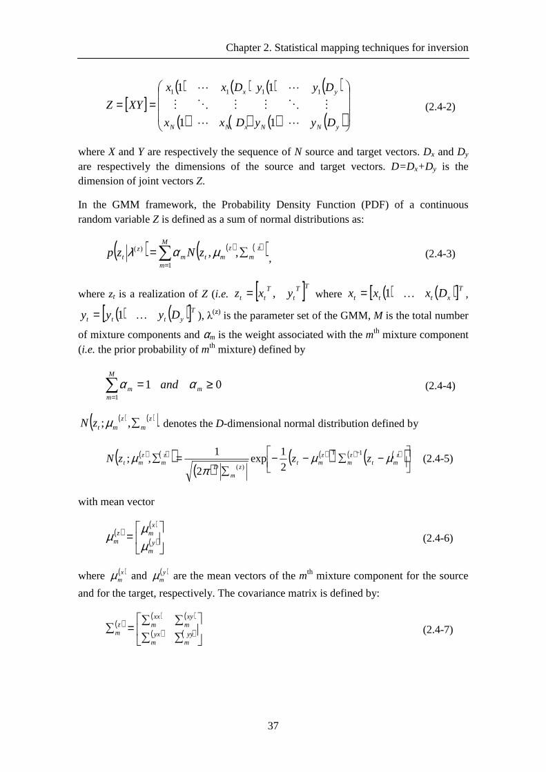
Chapter 2. Statistical mapping techniques for inversion
37
[ ]( ) ( )
( ) ( )
( ) ( )
( ) ( )
==
yNN
y
xNN
x
Dyy
Dyy
Dxx
Dxx
XYZ
L
MOM
L
L
MOM
L
1
1
1
1 1111
(2.4-2)
where X and Y are respectively the sequence of N source and target vectors. Dx and Dy are respectively the dimensions of the source and target vectors. D=Dx+Dy is the dimension of joint vectors Z.
In the GMM framework, the Probability Density Function (PDF) of a continuous random variable Z is defined as a sum of normal distributions as:
( ) ( ) ( )( )∑=
∑=M
m
zm
zmtm
zt zNzp
1
)( ,,µαλ , (2.4-3)
where zt is a realization of Z (i.e. [ ]TTt
Ttt yxz ,= where ( ) ( )[ ]Txttt Dxxx K1= ,
( ) ( )[ ]Tyttt Dyyy K1= ), λ(z) is the parameter set of the GMM, M is the total number
of mixture components and αm is the weight associated with the mth mixture component (i.e. the prior probability of mth mixture) defined by
∑=
≥=M
mmm and
1
01 αα (2.4-4)
( ) ( )( )zm
zmtzN ∑,;µ denotes the D-dimensional normal distribution defined by
( ) ( )( )( )
( )( ) ( ) ( )( )
−∑−−∑
=∑−Τ z
mtz
mz
mtz
mD
zm
zmt zzzN µµ
πµ 1
)( 2
1exp
2
1,; (2.4-5)
with mean vector
( )
( )
( )
=
ym
xmz
m µµµ (2.4-6)
where ( )xmµ and ( )y
mµ are the mean vectors of the mth mixture component for the source
and for the target, respectively. The covariance matrix is defined by:
( )
( ) ( )
( ) ( )
∑∑
∑∑=∑
yym
yxm
xym
xxmz
m (2.4-7)
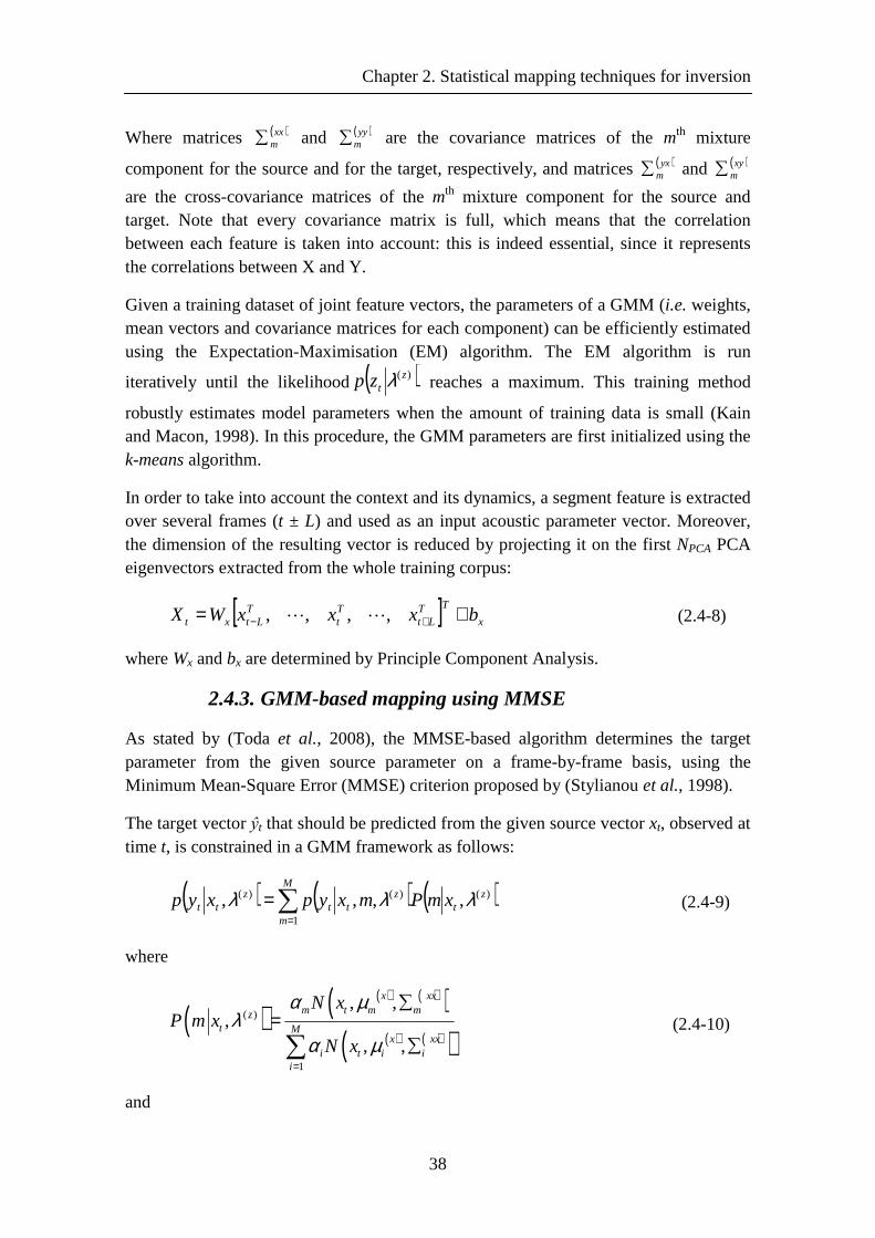
Chapter 2. Statistical mapping techniques for inversion
38
Where matrices ( )xxm∑ and ( )yy
m∑ are the covariance matrices of the mth mixture
component for the source and for the target, respectively, and matrices ( )yxm∑ and ( )xy
m∑
are the cross-covariance matrices of the mth mixture component for the source and target. Note that every covariance matrix is full, which means that the correlation between each feature is taken into account: this is indeed essential, since it represents the correlations between X and Y.
Given a training dataset of joint feature vectors, the parameters of a GMM (i.e. weights, mean vectors and covariance matrices for each component) can be efficiently estimated using the Expectation-Maximisation (EM) algorithm. The EM algorithm is run
iteratively until the likelihood ( ))(ztzp λ reaches a maximum. This training method
robustly estimates model parameters when the amount of training data is small (Kain and Macon, 1998). In this procedure, the GMM parameters are first initialized using the k-means algorithm.
In order to take into account the context and its dynamics, a segment feature is extracted over several frames (t ± L) and used as an input acoustic parameter vector. Moreover, the dimension of the resulting vector is reduced by projecting it on the first NPCA PCA eigenvectors extracted from the whole training corpus:
[ ] x
TTLt
Tt
TLtxt bxxxWX += +− ,,,, LL (2.4-8)
where Wx and bx are determined by Principle Component Analysis.
2.4.3. GMM-based mapping using MMSE
As stated by (Toda et al., 2008), the MMSE-based algorithm determines the target parameter from the given source parameter on a frame-by-frame basis, using the Minimum Mean-Square Error (MMSE) criterion proposed by (Stylianou et al., 1998).
The target vector ŷt that should be predicted from the given source vector xt, observed at time t, is constrained in a GMM framework as follows:
( ) ( ) ( )∑=
=M
m
zt
ztt
ztt xmPmxypxyp
1
)()()( ,,,, λλλ (2.4-9)
where
( )( ) ( )( )
( ) ( )( )( )
1
, ,,
, ,
x xxm t m mz
t Mx xx
i t i ii
N xP m x
N x
α µλ
α µ=
∑=
∑∑ (2.4-10)
and
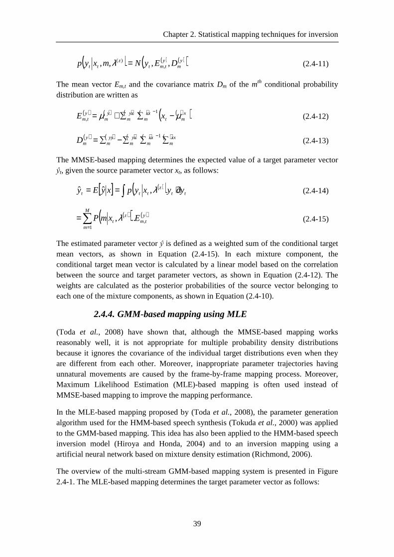
Chapter 2. Statistical mapping techniques for inversion
39
( ) ( ) ( )( )ym
ytmt
ztt DEyNmxyp ,,,, ,
)( =λ (2.4-11)
The mean vector Em,t and the covariance matrix Dm of the mth conditional probability distribution are written as
( ) ( ) ( ) ( ) ( )( )xmt
xxm
yxm
ym
ytm xE µµ −∑∑+= −1
, (2.4-12)
( ) ( ) ( ) ( ) ( )xxm
xxm
yxm
yym
ymD ∑∑∑−∑= −1
(2.4-13)
The MMSE-based mapping determines the expected value of a target parameter vector ŷt, given the source parameter vector xt, as follows:
[ ] ( )( ) ttz
ttt yyxypxyEy ∂⋅== ∫ λ,ˆˆ (2.4-14)
( )( ) ( )y
tm
M
m
zt ExmP ,
1
..,∑=
= λ (2.4-15)
The estimated parameter vector ŷ is defined as a weighted sum of the conditional target mean vectors, as shown in Equation (2.4-15). In each mixture component, the conditional target mean vector is calculated by a linear model based on the correlation between the source and target parameter vectors, as shown in Equation (2.4-12). The weights are calculated as the posterior probabilities of the source vector belonging to each one of the mixture components, as shown in Equation (2.4-10).
2.4.4. GMM-based mapping using MLE
(Toda et al., 2008) have shown that, although the MMSE-based mapping works reasonably well, it is not appropriate for multiple probability density distributions because it ignores the covariance of the individual target distributions even when they are different from each other. Moreover, inappropriate parameter trajectories having unnatural movements are caused by the frame-by-frame mapping process. Moreover, Maximum Likelihood Estimation (MLE)-based mapping is often used instead of MMSE-based mapping to improve the mapping performance.
In the MLE-based mapping proposed by (Toda et al., 2008), the parameter generation algorithm used for the HMM-based speech synthesis (Tokuda et al., 2000) was applied to the GMM-based mapping. This idea has also been applied to the HMM-based speech inversion model (Hiroya and Honda, 2004) and to an inversion mapping using a artificial neural network based on mixture density estimation (Richmond, 2006).
The overview of the multi-stream GMM-based mapping system is presented in Figure 2.4-1. The MLE-based mapping determines the target parameter vector as follows:
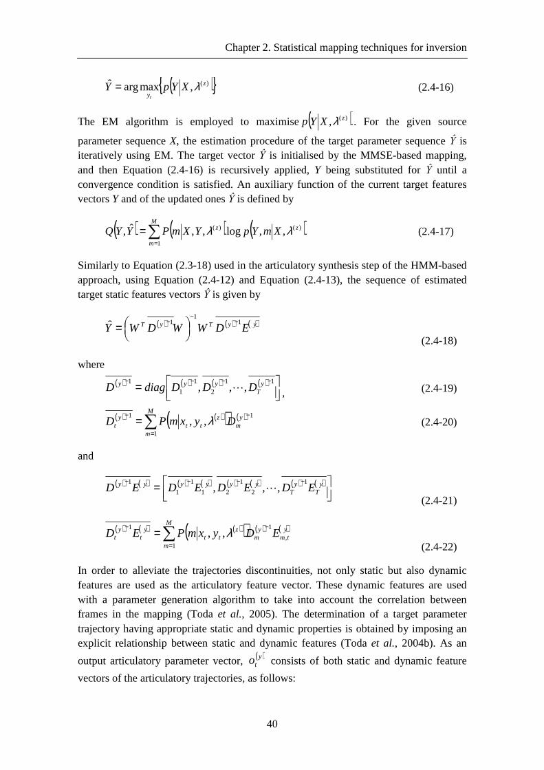
Chapter 2. Statistical mapping techniques for inversion
40
( ){ })(,maxargˆ z
yXYpY
t
λ= (2.4-16)
The EM algorithm is employed to maximise( ))(, zXYp λ . For the given source
parameter sequence X, the estimation procedure of the target parameter sequence Ŷ is iteratively using EM. The target vector Ŷ is initialised by the MMSE-based mapping, and then Equation (2.4-16) is recursively applied, Y being substituted for Ŷ until a convergence condition is satisfied. An auxiliary function of the current target features vectors Y and of the updated ones Ŷ is defined by
( ) ( ) ( )∑=
=M
m
zz XmYpYXmPYYQ1
)()( ,,log,,ˆ, λλ (2.4-17)
Similarly to Equation (2.3-18) used in the articulatory synthesis step of the HMM-based approach, using Equation (2.4-12) and Equation (2.4-13), the sequence of estimated target static features vectors Ŷ is given by
( ) ( ) ( )yyTyT EDWWDWY1
11ˆ −
−−
=
(2.4-18)
where
( ) ( ) ( ) ( )
= −−−− 11
2
1
1
1,,, y
Tyyy DDDdiagD L , (2.4-19)
( ) ( )( ) ( )∑
=
−−=
M
m
ym
ztt
yt DyxmPD
1
11,, λ (2.4-20)
and
( ) ( ) ( ) ( ) ( ) ( ) ( ) ( )
= −−−− y
Ty
Tyyyyyy EDEDEDED
1
2
1
21
1
1
1,,, L
(2.4-21)
( ) ( ) ( )( ) ( ) ( )∑=
−−=
M
m
ytm
ym
ztt
yt
yt EDyxmPED
1,
11,, λ
(2.4-22)
In order to alleviate the trajectories discontinuities, not only static but also dynamic features are used as the articulatory feature vector. These dynamic features are used with a parameter generation algorithm to take into account the correlation between frames in the mapping (Toda et al., 2005). The determination of a target parameter trajectory having appropriate static and dynamic properties is obtained by imposing an explicit relationship between static and dynamic features (Toda et al., 2004b). As an
output articulatory parameter vector, ( )yto consists of both static and dynamic feature
vectors of the articulatory trajectories, as follows:
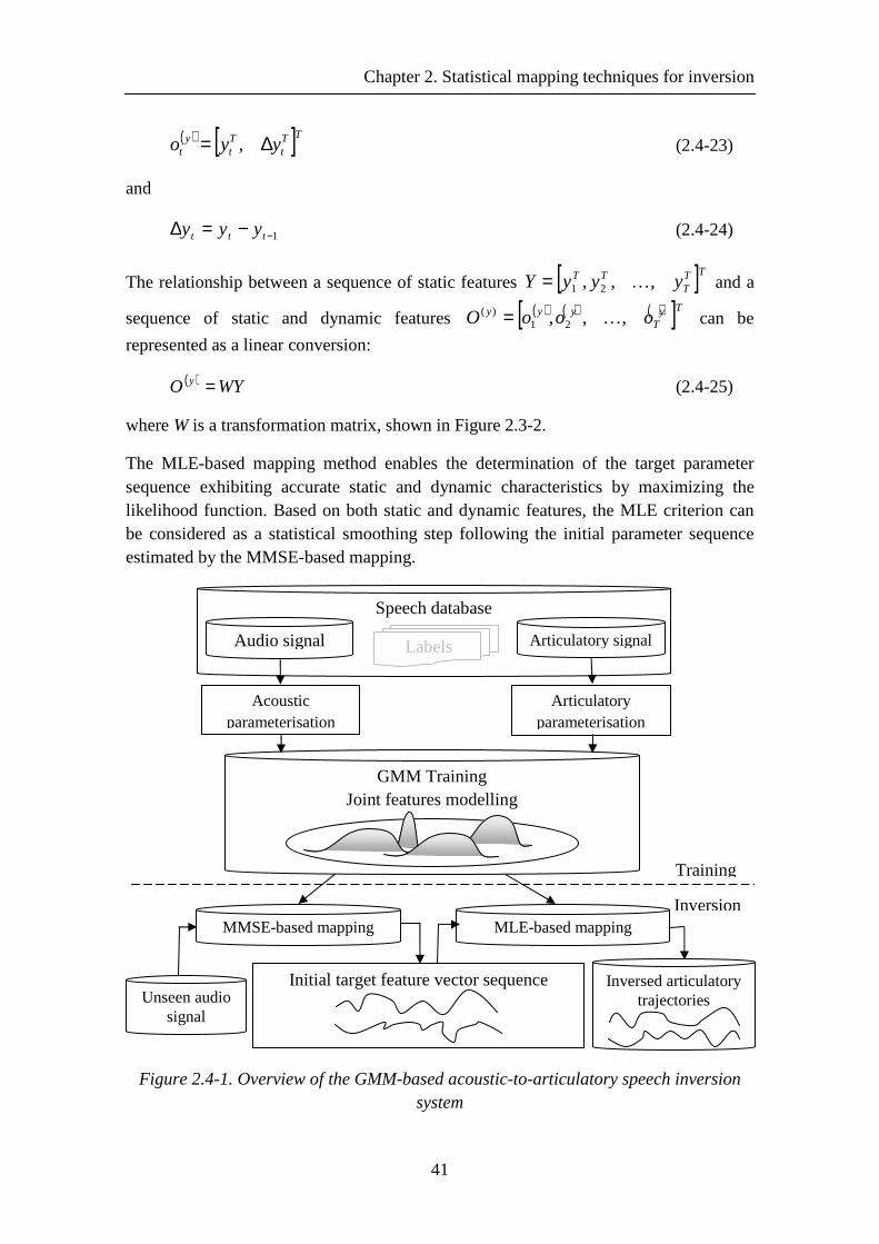
Chapter 2. Statistical mapping techniques for inversion
41
( ) [ ]TTt
Tt
yt yyo ∆= , (2.4-23)
and
1−−=∆ ttt yyy (2.4-24)
The relationship between a sequence of static features [ ]TTT
TT yyyY ,,, 21 K= and a
sequence of static and dynamic features ( ) ( ) ( )[ ]TyT
yyy oooO ,,, 21)(
K= can be
represented as a linear conversion:
( ) WYO y = (2.4-25)
where W is a transformation matrix, shown in Figure 2.3-2.
The MLE-based mapping method enables the determination of the target parameter sequence exhibiting accurate static and dynamic characteristics by maximizing the likelihood function. Based on both static and dynamic features, the MLE criterion can be considered as a statistical smoothing step following the initial parameter sequence estimated by the MMSE-based mapping.
Figure 2.4-1. Overview of the GMM-based acoustic-to-articulatory speech inversion system
Speech database Articulatory signal Audio signal Labels
GMM Training Joint features modelling
Articulatory parameterisation
Training
Acoustic parameterisation
Inversed articulatory trajectories
MLE-based mapping Inversion
Unseen audio signal
MMSE-based mapping
Initial target feature vector sequence
Chapter 2. Statistical mapping techniques for inversion
42
2.5. Summary
Various approaches of inversion mapping were found in the literature. In this chapter, we reviewed the state of the art of the acoustic-to-articulatory mapping and we choose the two different statistical techniques which give the best results in previous work: the first one is based on HMMs that use phonetic information as intermediate level between acoustic and articulatory stream compared to the second technique based on GMMs that maps directly the acoustic features to the articulatory ones. We have also presented the theory of statistical mapping based on HMMs and GMMs, as well as a description of some improvements of these techniques, such as the inheritance mechanism, the tied states, the increase of Gaussian mixtures, and the minimum generation error training for HMMs or maximum likelihood estimation criteria for GMMs.
To train and test statistical models such as HMMs or GMMs, real data are needed. In the next chapter we present the acoustic and articulatory data recorded and used in order to implement these methods.
Chapter 3. Acoustic and articulatory speech data
43
Chapter 3. Acoustic and articulatory speech data
3.1. Introduction
A crucial part of any statistical machine learning system is the data. Depending on the specific aim of the system, one first has to determine what kind of information must be present in the corpus to be collected. Two important issues are at stake in the construction of the speech corpus for our acoustic-to-articulatory system: (1) the database size, that refers to the amount of parallel acoustic and articulatory data available, should be large enough to allow reliable estimation of the statistical parameters; and (2) the phonetic coverage, that describes the extent of the speech utterances produced by the speaker, should encompass as much as possible the space of possible speech sounds in the language, such as phonemes, biphones or triphones.
To sum up, the recorded speech corpus should maximally represent all the articulatory movements and corresponding sounds which can be found in the language. The chosen sentences must cover maximally allophonic variations of each phoneme, i.e. the phonemes with their allophonic variations that depend on the right and left contexts. However, because the experimental settings require a short recording session and the speaker should not feel too much fatigue, the size of the corpus has to be limited.
In this thesis, two corpuses of one French speaker recorded under studio conditions and the English MOCHA-TIMIT corpus were used. The construction and the analysis of these corpuses will be presented in the next sections.
3.2. Methods for articulatory data acquisition
While acoustic speech signals can simply be recorded by means of a microphone, several methods have been proposed over the years to measure the vocal tract shape and movement.
3.2.1. X-ray cineradiography
X-ray cineradiography was used for the first time in the 1920’s (Russell, 1928). X-ray data were very useful to provide knowledge about the movements of the vocal tract. It has traditionally been the main source of information for movement of the shape and the position of the articulators during speech. The advantage of x-ray imaging is that it
Chapter 3. Acoustic and articulatory speech data
44
provides images of good resolution at a rate of about 50 images / sec. for the entire head, while the speaker can sit in upright position. A difficulty with x-rays is to accurately identify the vocal tract structures in the images, which are actually constituted by the projection of the different head structures on a sagittal plane. To enhance the contrast in the images, subjects swallow a viscous liquid containing a contrast agent (barium for instance) that adheres to the surface of tongue, mouth floor and to lips. The limited exposure radiation time is another severe limitation on the usefulness of x-ray films.
3.2.2. X-ray microbeam cinematography
In order to reduce the risks of x-ray radiation, Kiritani (1986) and his team has developed the x-ray microbeam system that uses a narrow beam of x-ray controlled by computer to localise and track the movements of small gold pellets attached to the speakers’ articulators. This method offers a good time resolution and covers the whole vocal tract but does not provide 3D images. Although this system reduces the time of subject’s exposure under x-ray, it has now been largely replaced by safer methods such as ElectroMagnetic Articulography.
3.2.3. Magnetic Resonance Imaging
Magnetic Resonance Imaging (MRI) can provide detailed data of the entire vocal tract and tongue without any known dangerous effects on the subject. The images are amenable to computerized 3D modelling. In addition, the vocal tract area and volume can be directly calculated. Because of its extremely slow acquisition speed, the subject often has to maintain the articulation for several seconds. Thanks to technical advances, it is nowadays possible to collect full 3D data of speech articulation. However, the rate of images is still not high enough to observe natural articulatory movements. In addition, the quality of images is rather low. Another drawback of MRI is that the subjects have to be positioned in supine position lying on their back, due to the construction of the MRI scanner and antenna. The gravitational effects of this positioning might have some influence on the articulation (Tiede et al., 2000; Stone et al., 2007). Even if MRI imaging does not offer a sufficient fast sampling rate, it provides 3D images of the vocal tract with a good spatial resolution. It is thus now widely used to collect still images and derive 3D vocal tract geometry from these images (Engwall, 2000).
3.2.4. Ultrasound echography
Another technique for capturing the articulatory movements of tongue is the ultrasound echography (cf. (Stone et al. (1983; 1990)). Ultrasound is an ultra high-frequency sound wave that is directed through the lingual soft tissue. Some of the emitted sound waves from the transducer are reflected back when they reach the tongue-air boundary on the superior surface of the tongue, and return to the same transducer. The shape of the
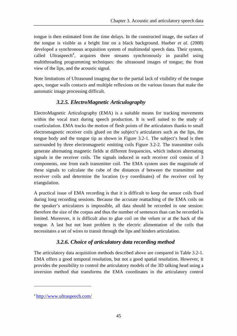
Chapter 3. Acoustic and articulatory speech data
45
tongue is then estimated from the time delays. In the constructed image, the surface of the tongue is visible as a bright line on a black background. Hueber et al. (2008) developed a synchronous acquisition system of multimodal speech data. Their system, called Ultraspeech4, acquires three streams synchronously in parallel using multithreading programming techniques: the ultrasound images of tongue; the front view of the lips, and the acoustic signal.
Note limitations of Ultrasound imaging due to the partial lack of visibility of the tongue apex, tongue walls contacts and multiple reflexions on the various tissues that make the automatic image processing difficult.
3.2.5. ElectroMagnetic Articulography
ElectroMagnetic Articulography (EMA) is a suitable means for tracking movements within the vocal tract during speech production. It is well suited to the study of coarticulation. EMA tracks the motion of flesh points of the articulators thanks to small electromagnetic receiver coils glued on the subject’s articulators such as the lips, the tongue body and the tongue tip as shown in Figure 3.2-1. The subject’s head is then surrounded by three electromagnetic emitting coils Figure 3.2-2. The transmitter coils generate alternating magnetic fields at different frequencies, which induces alternating signals in the receiver coils. The signals induced in each receiver coil consist of 3 components, one from each transmitter coil. The EMA system uses the magnitude of these signals to calculate the cube of the distances d between the transmitter and receiver coils and determine the location (x-y coordinates) of the receiver coil by triangulation.
A practical issue of EMA recording is that it is difficult to keep the sensor coils fixed during long recording sessions. Because the accurate reattaching of the EMA coils on the speaker’s articulators is impossible, all data should be recorded in one session: therefore the size of the corpus and thus the number of sentences than can be recorded is limited. Moreover, it is difficult also to glue coil on the velum or at the back of the tongue. A last but not least problem is the electric alimentation of the coils that necessitates a set of wires to transit through the lips and hinders articulation.
3.2.6. Choice of articulatory data recording method
The articulatory data acquisition methods described above are compared in Table 3.2-1. EMA offers a good temporal resolution, but not a good spatial resolution. However, it provides the possibility to control the articulatory models of the 3D talking head using a inversion method that transforms the EMA coordinates in the articulatory control
4 http://www.ultraspeech.com/
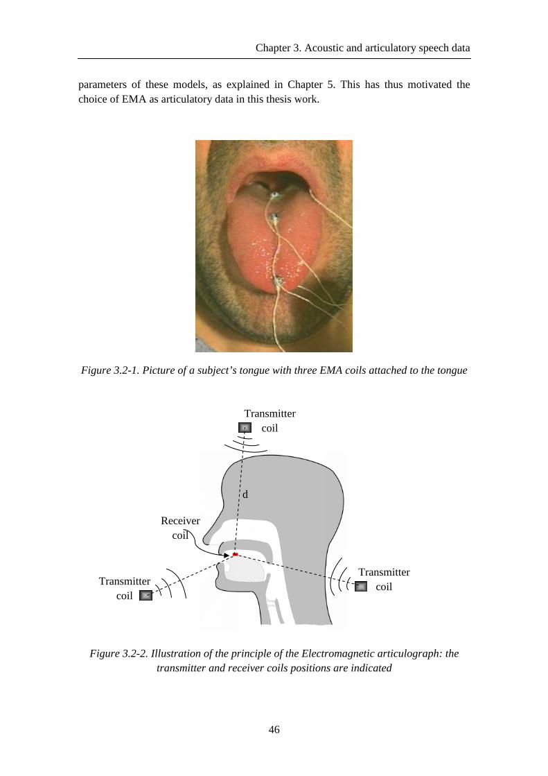
Chapter 3. Acoustic and articulatory speech data
46
parameters of these models, as explained in Chapter 5. This has thus motivated the choice of EMA as articulatory data in this thesis work.
Figure 3.2-1. Picture of a subject’s tongue with three EMA coils attached to the tongue
Figure 3.2-2. Illustration of the principle of the Electromagnetic articulograph: the transmitter and receiver coils positions are indicated
Receiver coil
Transmitter coil
Transmitter coil
Transmitter coil
d
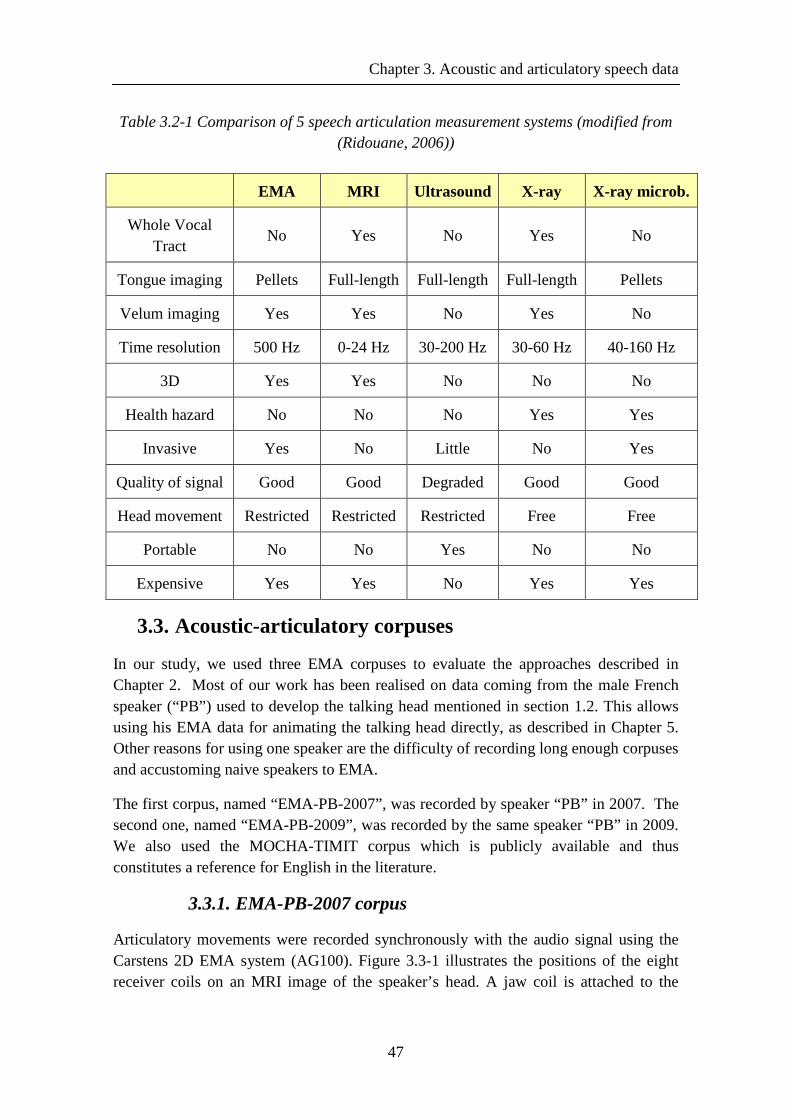
Chapter 3. Acoustic and articulatory speech data
47
Table 3.2-1 Comparison of 5 speech articulation measurement systems (modified from (Ridouane, 2006))
EMA MRI Ultrasound X-ray X-ray microb.
Whole Vocal Tract
No Yes No Yes No
Tongue imaging Pellets Full-length Full-length Full-length Pellets
Velum imaging Yes Yes No Yes No
Time resolution 500 Hz 0-24 Hz 30-200 Hz 30-60 Hz 40-160 Hz
3D Yes Yes No No No
Health hazard No No No Yes Yes
Invasive Yes No Little No Yes
Quality of signal Good Good Degraded Good Good
Head movement Restricted Restricted Restricted Free Free
Portable No No Yes No No
Expensive Yes Yes No Yes Yes
3.3. Acoustic-articulatory corpuses
In our study, we used three EMA corpuses to evaluate the approaches described in Chapter 2. Most of our work has been realised on data coming from the male French speaker (“PB”) used to develop the talking head mentioned in section 1.2. This allows using his EMA data for animating the talking head directly, as described in Chapter 5. Other reasons for using one speaker are the difficulty of recording long enough corpuses and accustoming naive speakers to EMA.
The first corpus, named “EMA-PB-2007”, was recorded by speaker “PB” in 2007. The second one, named “EMA-PB-2009”, was recorded by the same speaker “PB” in 2009. We also used the MOCHA-TIMIT corpus which is publicly available and thus constitutes a reference for English in the literature.
3.3.1. EMA-PB-2007 corpus
Articulatory movements were recorded synchronously with the audio signal using the Carstens 2D EMA system (AG100). Figure 3.3-1 illustrates the positions of the eight receiver coils on an MRI image of the speaker’s head. A jaw coil is attached to the
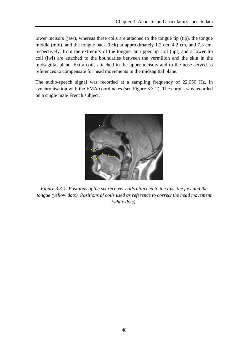
Chapter 3. Acoustic and articulatory speech data
48
lower incisors (jaw), whereas three coils are attached to the tongue tip (tip), the tongue middle (mid), and the tongue back (bck) at approximately 1.2 cm, 4.2 cm, and 7.3 cm, respectively, from the extremity of the tongue; an upper lip coil (upl) and a lower lip coil (lwl) are attached to the boundaries between the vermilion and the skin in the midsagittal plane. Extra coils attached to the upper incisors and to the nose served as references to compensate for head movements in the midsagittal plane.
The audio-speech signal was recorded at a sampling frequency of 22,050 Hz, in synchronisation with the EMA coordinates (see Figure 3.3-2). The corpus was recorded on a single male French subject.
Figure 3.3-1. Positions of the six receiver coils attached to the lips, the jaw and the tongue (yellow dots). Positions of coils used as reference to correct the head movement
(white dots).
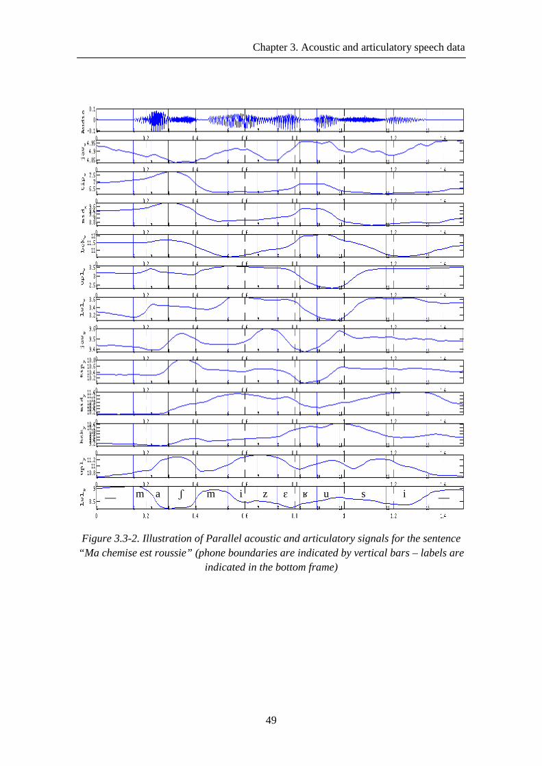
Chapter 3. Acoustic and articulatory speech data
49
Figure 3.3-2. Illustration of Parallel acoustic and articulatory signals for the sentence “Ma chemise est roussie” (phone boundaries are indicated by vertical bars – labels are
indicated in the bottom frame)
__ m m a ʃ i z ɛ ʁ u s i __
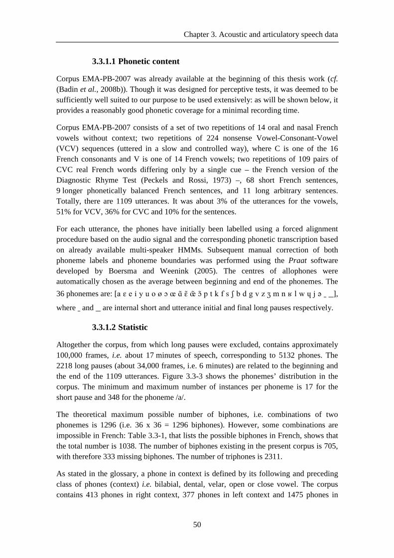
Chapter 3. Acoustic and articulatory speech data
50
3.3.1.1 Phonetic content
Corpus EMA-PB-2007 was already available at the beginning of this thesis work (cf. (Badin et al., 2008b)). Though it was designed for perceptive tests, it was deemed to be sufficiently well suited to our purpose to be used extensively: as will be shown below, it provides a reasonably good phonetic coverage for a minimal recording time.
Corpus EMA-PB-2007 consists of a set of two repetitions of 14 oral and nasal French vowels without context; two repetitions of 224 nonsense Vowel-Consonant-Vowel (VCV) sequences (uttered in a slow and controlled way), where C is one of the 16 French consonants and V is one of 14 French vowels; two repetitions of 109 pairs of CVC real French words differing only by a single cue – the French version of the Diagnostic Rhyme Test (Peckels and Rossi, 1973) –, 68 short French sentences, 9 longer phonetically balanced French sentences, and 11 long arbitrary sentences. Totally, there are 1109 utterances. It was about 3% of the utterances for the vowels, 51% for VCV, 36% for CVC and 10% for the sentences.
For each utterance, the phones have initially been labelled using a forced alignment procedure based on the audio signal and the corresponding phonetic transcription based on already available multi-speaker HMMs. Subsequent manual correction of both phoneme labels and phoneme boundaries was performed using the Praat software developed by Boersma and Weenink (2005). The centres of allophones were automatically chosen as the average between beginning and end of the phonemes. The
36 phonemes are: [a ɛ e i y u o ø ɔ œ ɑ ̃ɛ ̃œ̃ ɔ ̃p t k f s ʃ b d g v z ʒ m n ʁ l w ɥ j ə _ __],
where _ and __ are internal short and utterance initial and final long pauses respectively.
3.3.1.2 Statistic
Altogether the corpus, from which long pauses were excluded, contains approximately 100,000 frames, i.e. about 17 minutes of speech, corresponding to 5132 phones. The 2218 long pauses (about 34,000 frames, i.e. 6 minutes) are related to the beginning and the end of the 1109 utterances. Figure 3.3-3 shows the phonemes’ distribution in the corpus. The minimum and maximum number of instances per phoneme is 17 for the short pause and 348 for the phoneme /a/.
The theoretical maximum possible number of biphones, i.e. combinations of two phonemes is 1296 (i.e. 36 x 36 = 1296 biphones). However, some combinations are impossible in French: Table 3.3-1, that lists the possible biphones in French, shows that the total number is 1038. The number of biphones existing in the present corpus is 705, with therefore 333 missing biphones. The number of triphones is 2311.
As stated in the glossary, a phone in context is defined by its following and preceding class of phones (context) i.e. bilabial, dental, velar, open or close vowel. The corpus contains 413 phones in right context, 377 phones in left context and 1475 phones in
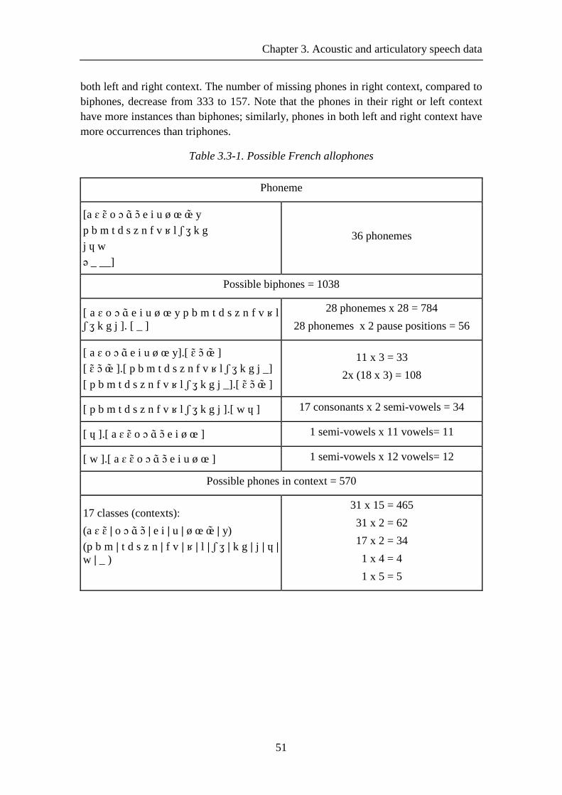
Chapter 3. Acoustic and articulatory speech data
51
both left and right context. The number of missing phones in right context, compared to biphones, decrease from 333 to 157. Note that the phones in their right or left context have more instances than biphones; similarly, phones in both left and right context have more occurrences than triphones.
Table 3.3-1. Possible French allophones
Phoneme
[a ɛ ɛ ̃o ɔ ɑ̃ ɔ̃ e i u ø œ œ̃ y
p b m t d s z n f v ʁ l ʃ ʒ k g
j ɥ w
ə _ __]
36 phonemes
Possible biphones = 1038
[ a ɛ o ɔ ɑ̃ e i u ø œ y p b m t d s z n f v ʁ l ʃ ʒ k g j ]. [ _ ]
28 phonemes x 28 = 784
28 phonemes x 2 pause positions = 56
[ a ɛ o ɔ ɑ̃ e i u ø œ y].[ ɛ ̃ɔ̃ œ̃ ]
[ ɛ ̃ɔ̃ œ̃ ].[ p b m t d s z n f v ʁ l ʃ ʒ k g j _]
[ p b m t d s z n f v ʁ l ʃ ʒ k g j _].[ ɛ ̃ɔ̃ œ̃ ]
11 x 3 = 33
2x (18 x 3) = 108
[ p b m t d s z n f v ʁ l ʃ ʒ k g j ].[ w ɥ ] 17 consonants x 2 semi-vowels = 34
[ ɥ ].[ a ɛ ɛ ̃o ɔ ɑ̃ ɔ̃ e i ø œ ] 1 semi-vowels x 11 vowels= 11
[ w ].[ a ɛ ɛ ̃o ɔ ɑ̃ ɔ̃ e i u ø œ ] 1 semi-vowels x 12 vowels= 12
Possible phones in context = 570
17 classes (contexts):
(a ɛ ɛ ̃| o ɔ ɑ̃ ɔ̃ | e i | u | ø œ œ̃ | y)
(p b m | t d s z n | f v | ʁ | l | ʃ ʒ | k g | j | ɥ | w | _ )
31 x 15 = 465
31 x 2 = 62
17 x 2 = 34
1 x 4 = 4
1 x 5 = 5
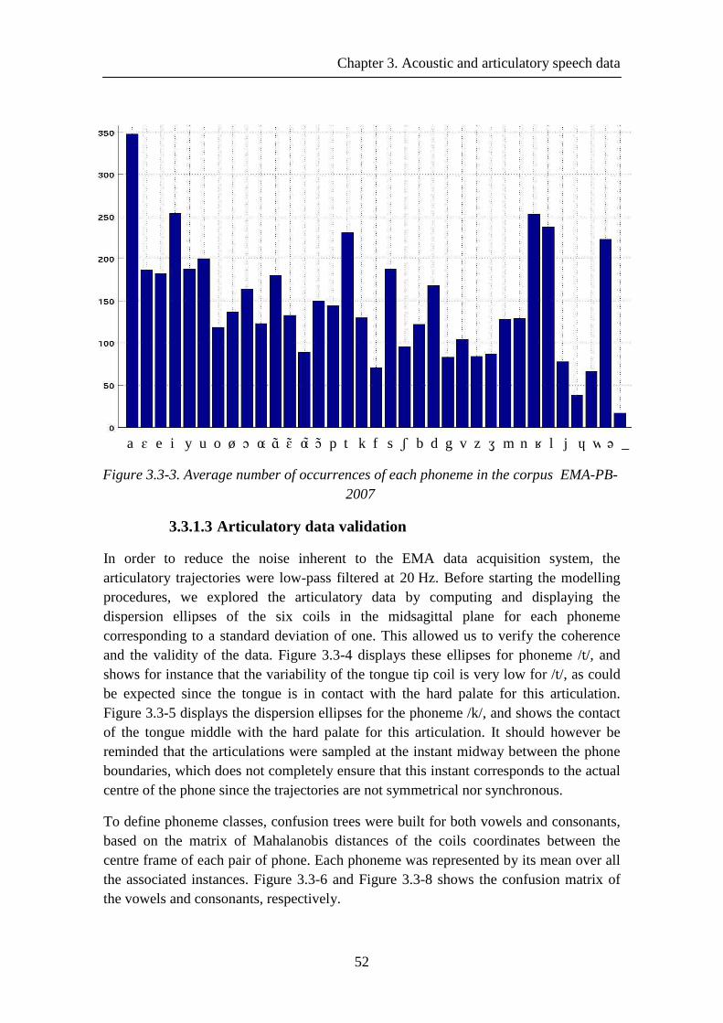
Chapter 3. Acoustic and articulatory speech data
52
3.3.1.3 Articulatory data validation
In order to reduce the noise inherent to the EMA data acquisition system, the articulatory trajectories were low-pass filtered at 20 Hz. Before starting the modelling procedures, we explored the articulatory data by computing and displaying the dispersion ellipses of the six coils in the midsagittal plane for each phoneme corresponding to a standard deviation of one. This allowed us to verify the coherence and the validity of the data. Figure 3.3-4 displays these ellipses for phoneme /t/, and shows for instance that the variability of the tongue tip coil is very low for /t/, as could be expected since the tongue is in contact with the hard palate for this articulation. Figure 3.3-5 displays the dispersion ellipses for the phoneme /k/, and shows the contact of the tongue middle with the hard palate for this articulation. It should however be reminded that the articulations were sampled at the instant midway between the phone boundaries, which does not completely ensure that this instant corresponds to the actual centre of the phone since the trajectories are not symmetrical nor synchronous.
To define phoneme classes, confusion trees were built for both vowels and consonants, based on the matrix of Mahalanobis distances of the coils coordinates between the centre frame of each pair of phone. Each phoneme was represented by its mean over all the associated instances. Figure 3.3-6 and Figure 3.3-8 shows the confusion matrix of the vowels and consonants, respectively.
a ɛ e i y u o ø ɔ œɑ̃ ɛ ̃ œ̃ɔ̃ p t k f s ʃ b d g v z ʒ m n ʁ l j ɥ w ə _
Figure 3.3-3. Average number of occurrences of each phoneme in the corpus EMA-PB-2007
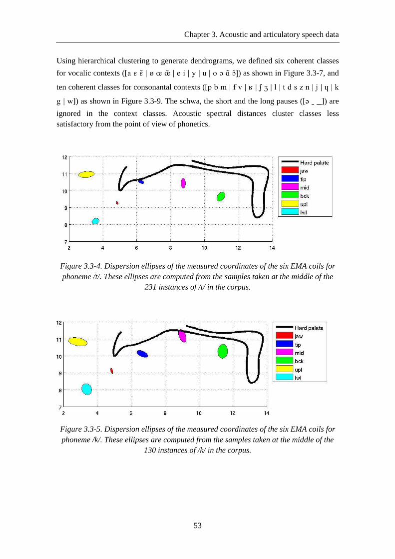
Chapter 3. Acoustic and articulatory speech data
53
Using hierarchical clustering to generate dendrograms, we defined six coherent classes
for vocalic contexts ([a ɛ ɛ ̃| ø œ œ̃ | e i | y | u | o ɔ ɑ ̃ɔ]̃) as shown in Figure 3.3-7, and
ten coherent classes for consonantal contexts ([p b m | f v | ʁ | ʃ ʒ | l | t d s z n | j | ɥ | k
g | w]) as shown in Figure 3.3-9. The schwa, the short and the long pauses ([ə _ __]) are
ignored in the context classes. Acoustic spectral distances cluster classes less satisfactory from the point of view of phonetics.
Figure 3.3-4. Dispersion ellipses of the measured coordinates of the six EMA coils for phoneme /t/. These ellipses are computed from the samples taken at the middle of the
231 instances of /t/ in the corpus.
Figure 3.3-5. Dispersion ellipses of the measured coordinates of the six EMA coils for phoneme /k/. These ellipses are computed from the samples taken at the middle of the
130 instances of /k/ in the corpus.
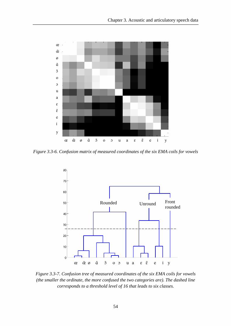
Chapter 3. Acoustic and articulatory speech data
54
œ
œ̃
ø
ɑ ̃
ɔ ̃
o
ɔ
u
a
ɛ
ɛ ̃
e
i
y
œ œ̃ ø ɑ ̃ ɔ ̃ o ɔ u a ɛ ɛ ̃ e i y
Figure 3.3-6. Confusion matrix of measured coordinates of the six EMA coils for vowels
œ œ̃ ø ɑ ̃ ɔ ̃ o ɔ u a ɛ ɛ ̃ e i y
Figure 3.3-7. Confusion tree of measured coordinates of the six EMA coils for vowels (the smaller the ordinate, the more confused the two categories are). The dashed line
corresponds to a threshold level of 16 that leads to six classes.
Rounded Unrounded
Front rounded
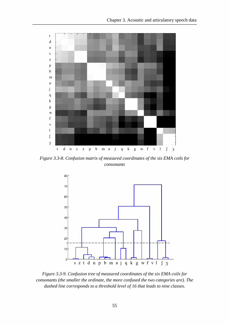
Chapter 3. Acoustic and articulatory speech data
55
t
d
n
s
z
p
b
m
ʁ
j
ɥ
k
g
w
f
v
l
ʃ
ʒ
t d n s z p b m ʁ j ɥ k g w f v l ʃ ʒ
Figure 3.3-8. Confusion matrix of measured coordinates of the six EMA coils for consonants
s z t d n p b m ʁ j ɥ k g w f v l ʃ ʒ
Figure 3.3-9. Confusion tree of measured coordinates of the six EMA coils for consonants (the smaller the ordinate, the more confused the two categories are). The
dashed line corresponds to a threshold level of 16 that leads to nine classes.
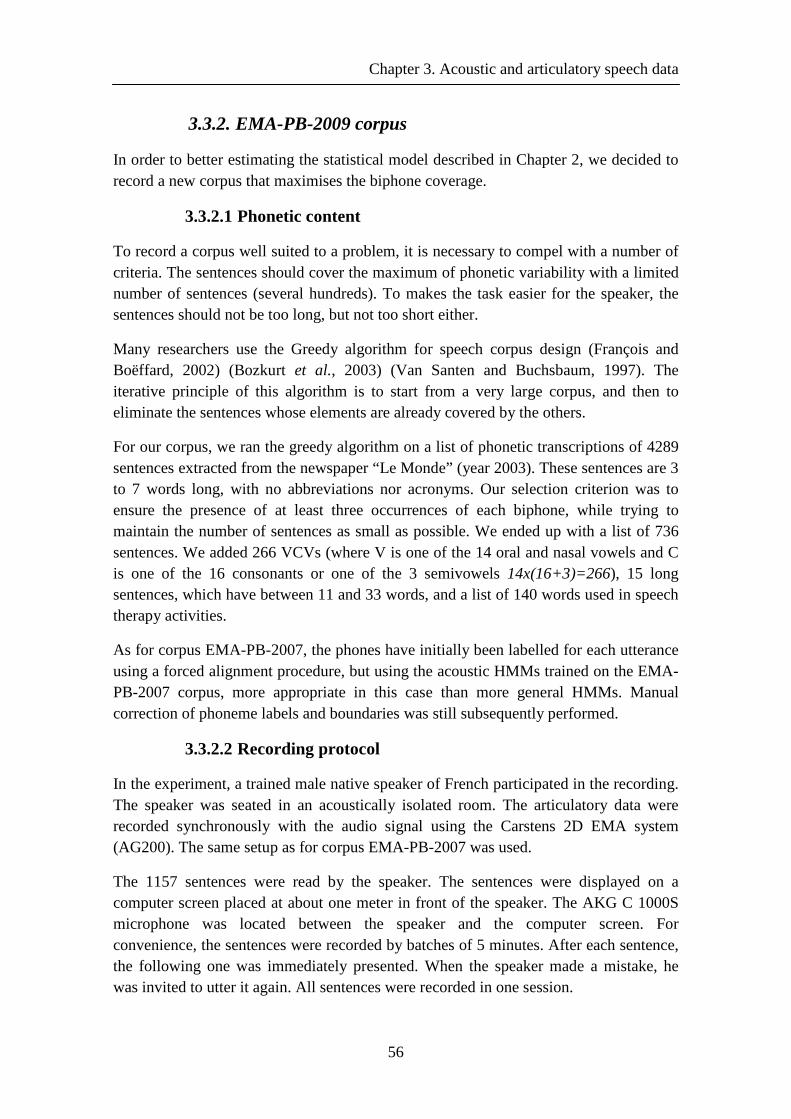
Chapter 3. Acoustic and articulatory speech data
56
3.3.2. EMA-PB-2009 corpus
In order to better estimating the statistical model described in Chapter 2, we decided to record a new corpus that maximises the biphone coverage.
3.3.2.1 Phonetic content
To record a corpus well suited to a problem, it is necessary to compel with a number of criteria. The sentences should cover the maximum of phonetic variability with a limited number of sentences (several hundreds). To makes the task easier for the speaker, the sentences should not be too long, but not too short either.
Many researchers use the Greedy algorithm for speech corpus design (François and Boëffard, 2002) (Bozkurt et al., 2003) (Van Santen and Buchsbaum, 1997). The iterative principle of this algorithm is to start from a very large corpus, and then to eliminate the sentences whose elements are already covered by the others.
For our corpus, we ran the greedy algorithm on a list of phonetic transcriptions of 4289 sentences extracted from the newspaper “Le Monde” (year 2003). These sentences are 3 to 7 words long, with no abbreviations nor acronyms. Our selection criterion was to ensure the presence of at least three occurrences of each biphone, while trying to maintain the number of sentences as small as possible. We ended up with a list of 736 sentences. We added 266 VCVs (where V is one of the 14 oral and nasal vowels and C is one of the 16 consonants or one of the 3 semivowels 14x(16+3)=266), 15 long sentences, which have between 11 and 33 words, and a list of 140 words used in speech therapy activities.
As for corpus EMA-PB-2007, the phones have initially been labelled for each utterance using a forced alignment procedure, but using the acoustic HMMs trained on the EMA-PB-2007 corpus, more appropriate in this case than more general HMMs. Manual correction of phoneme labels and boundaries was still subsequently performed.
3.3.2.2 Recording protocol
In the experiment, a trained male native speaker of French participated in the recording. The speaker was seated in an acoustically isolated room. The articulatory data were recorded synchronously with the audio signal using the Carstens 2D EMA system (AG200). The same setup as for corpus EMA-PB-2007 was used.
The 1157 sentences were read by the speaker. The sentences were displayed on a computer screen placed at about one meter in front of the speaker. The AKG C 1000S microphone was located between the speaker and the computer screen. For convenience, the sentences were recorded by batches of 5 minutes. After each sentence, the following one was immediately presented. When the speaker made a mistake, he was invited to utter it again. All sentences were recorded in one session.
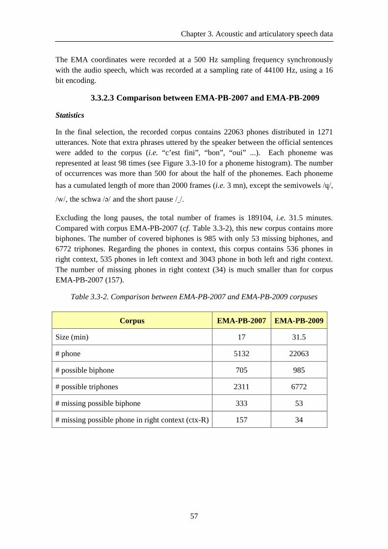
Chapter 3. Acoustic and articulatory speech data
57
The EMA coordinates were recorded at a 500 Hz sampling frequency synchronously with the audio speech, which was recorded at a sampling rate of 44100 Hz, using a 16 bit encoding.
3.3.2.3 Comparison between EMA-PB-2007 and EMA-PB-2009
Statistics
In the final selection, the recorded corpus contains 22063 phones distributed in 1271 utterances. Note that extra phrases uttered by the speaker between the official sentences were added to the corpus (i.e. “c’est fini”, “bon”, “oui” ...). Each phoneme was represented at least 98 times (see Figure 3.3-10 for a phoneme histogram). The number of occurrences was more than 500 for about the half of the phonemes. Each phoneme
has a cumulated length of more than 2000 frames (i.e. 3 mn), except the semivowels /ɥ/,
/w/, the schwa /ə/ and the short pause /_/.
Excluding the long pauses, the total number of frames is 189104, i.e. 31.5 minutes. Compared with corpus EMA-PB-2007 (cf. Table 3.3-2), this new corpus contains more biphones. The number of covered biphones is 985 with only 53 missing biphones, and 6772 triphones. Regarding the phones in context, this corpus contains 536 phones in right context, 535 phones in left context and 3043 phone in both left and right context. The number of missing phones in right context (34) is much smaller than for corpus EMA-PB-2007 (157).
Table 3.3-2. Comparison between EMA-PB-2007 and EMA-PB-2009 corpuses
Corpus EMA-PB-2007 EMA-PB-2009
Size (min) 17 31.5
# phone 5132 22063
# possible biphone 705 985
# possible triphones 2311 6772
# missing possible biphone 333 53
# missing possible phone in right context (ctx-R) 157 34
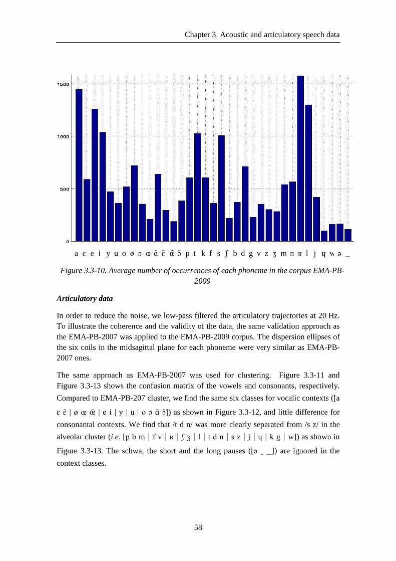
Chapter 3. Acoustic and articulatory speech data
58
Articulatory data
In order to reduce the noise, we low-pass filtered the articulatory trajectories at 20 Hz. To illustrate the coherence and the validity of the data, the same validation approach as the EMA-PB-2007 was applied to the EMA-PB-2009 corpus. The dispersion ellipses of the six coils in the midsagittal plane for each phoneme were very similar as EMA-PB-2007 ones.
The same approach as EMA-PB-2007 was used for clustering. Figure 3.3-11 and Figure 3.3-13 shows the confusion matrix of the vowels and consonants, respectively.
Compared to EMA-PB-207 cluster, we find the same six classes for vocalic contexts ([a
ɛ ɛ ̃ | ø œ œ̃ | e i | y | u | o ɔ ɑ ̃ɔ]̃) as shown in Figure 3.3-12, and little difference for
consonantal contexts. We find that /t d n/ was more clearly separated from /s z/ in the
alveolar cluster (i.e. [p b m | f v | ʁ | ʃ ʒ | l | t d n | s z | j | ɥ | k g | w]) as shown in
Figure 3.3-13. The schwa, the short and the long pauses ([ə _ __]) are ignored in the
context classes.
a ɛ e i y u o ø ɔ œɑ̃ ɛ ̃ œ̃ɔ̃ p t k f s ʃ b d g v z ʒ m n ʁ l j ɥ w ə _
Figure 3.3-10. Average number of occurrences of each phoneme in the corpus EMA-PB-2009
Chapter 3. Acoustic and articulatory speech data
59
œ
œ̃
ø
ɑ ̃
ɔ ̃
o
ɔ
u
a
ɛ
ɛ ̃
e
i
y
œ œ̃ ø ɑ ̃ ɔ ̃ o ɔ u a ɛ ɛ ̃ e i y
Figure 3.3-11. Confusion matrix of vowels in EMA-PB-2009 corpus
œ œ̃ ø ɑ ̃ ɔ ̃ o ɔ u y a
ɛ ɛ ̃ e
i
Figure 3.3-12. Confusion tree of articulatory parameters of vowels in EMA-PB-2009 corpus (the smaller ordinate, the more confused the two categories are). The dashed
line corresponds to a threshold level of 10 that leads to six classes.
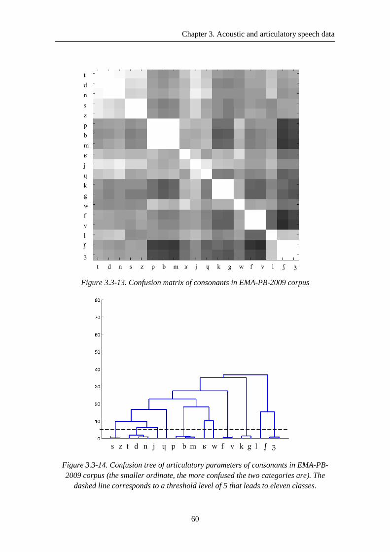
Chapter 3. Acoustic and articulatory speech data
60
t
d
n
s
z
p
b
m
ʁ
j
ɥ
k
g
w
f
v
l
ʃ
ʒ
t d n s z p b m ʁ j ɥ k g w f v l ʃ ʒ
Figure 3.3-13. Confusion matrix of consonants in EMA-PB-2009 corpus
s z t d n j ɥ
p
b
m ʁ w
f v
k
g l ʃ ʒ
Figure 3.3-14. Confusion tree of articulatory parameters of consonants in EMA-PB-2009 corpus (the smaller ordinate, the more confused the two categories are). The
dashed line corresponds to a threshold level of 5 that leads to eleven classes.
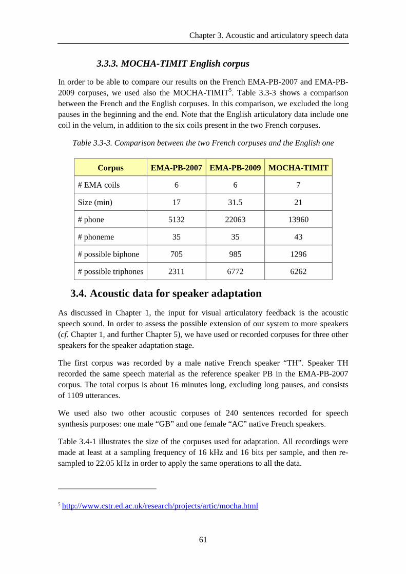
Chapter 3. Acoustic and articulatory speech data
61
3.3.3. MOCHA-TIMIT English corpus
In order to be able to compare our results on the French EMA-PB-2007 and EMA-PB-2009 corpuses, we used also the MOCHA-TIMIT5. Table 3.3-3 shows a comparison between the French and the English corpuses. In this comparison, we excluded the long pauses in the beginning and the end. Note that the English articulatory data include one coil in the velum, in addition to the six coils present in the two French corpuses.
Table 3.3-3. Comparison between the two French corpuses and the English one
Corpus EMA-PB-2007 EMA-PB-2009 MOCHA-TIMIT
# EMA coils 6 6 7
Size (min) 17 31.5 21
# phone 5132 22063 13960
# phoneme 35 35 43
# possible biphone 705 985 1296
# possible triphones 2311 6772 6262
3.4. Acoustic data for speaker adaptation
As discussed in Chapter 1, the input for visual articulatory feedback is the acoustic speech sound. In order to assess the possible extension of our system to more speakers (cf. Chapter 1, and further Chapter 5), we have used or recorded corpuses for three other speakers for the speaker adaptation stage.
The first corpus was recorded by a male native French speaker “TH”. Speaker TH recorded the same speech material as the reference speaker PB in the EMA-PB-2007 corpus. The total corpus is about 16 minutes long, excluding long pauses, and consists of 1109 utterances.
We used also two other acoustic corpuses of 240 sentences recorded for speech synthesis purposes: one male “GB” and one female “AC” native French speakers.
Table 3.4-1 illustrates the size of the corpuses used for adaptation. All recordings were made at least at a sampling frequency of 16 kHz and 16 bits per sample, and then re-sampled to 22.05 kHz in order to apply the same operations to all the data.
5 http://www.cstr.ed.ac.uk/research/projects/artic/mocha.html
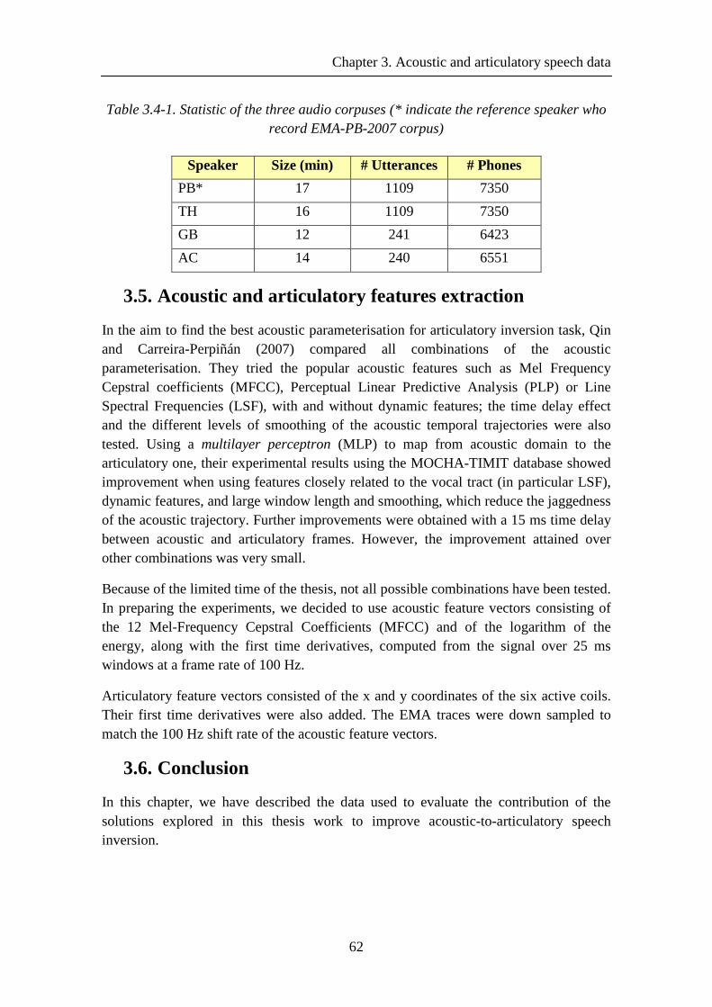
Chapter 3. Acoustic and articulatory speech data
62
Table 3.4-1. Statistic of the three audio corpuses (* indicate the reference speaker who record EMA-PB-2007 corpus)
Speaker Size (min) # Utterances # Phones
PB* 17 1109 7350
TH 16 1109 7350
GB 12 241 6423
AC 14 240 6551
3.5. Acoustic and articulatory features extraction
In the aim to find the best acoustic parameterisation for articulatory inversion task, Qin and Carreira-Perpiñán (2007) compared all combinations of the acoustic parameterisation. They tried the popular acoustic features such as Mel Frequency Cepstral coefficients (MFCC), Perceptual Linear Predictive Analysis (PLP) or Line Spectral Frequencies (LSF), with and without dynamic features; the time delay effect and the different levels of smoothing of the acoustic temporal trajectories were also tested. Using a multilayer perceptron (MLP) to map from acoustic domain to the articulatory one, their experimental results using the MOCHA-TIMIT database showed improvement when using features closely related to the vocal tract (in particular LSF), dynamic features, and large window length and smoothing, which reduce the jaggedness of the acoustic trajectory. Further improvements were obtained with a 15 ms time delay between acoustic and articulatory frames. However, the improvement attained over other combinations was very small.
Because of the limited time of the thesis, not all possible combinations have been tested. In preparing the experiments, we decided to use acoustic feature vectors consisting of the 12 Mel-Frequency Cepstral Coefficients (MFCC) and of the logarithm of the energy, along with the first time derivatives, computed from the signal over 25 ms windows at a frame rate of 100 Hz.
Articulatory feature vectors consisted of the x and y coordinates of the six active coils. Their first time derivatives were also added. The EMA traces were down sampled to match the 100 Hz shift rate of the acoustic feature vectors.
3.6. Conclusion
In this chapter, we have described the data used to evaluate the contribution of the solutions explored in this thesis work to improve acoustic-to-articulatory speech inversion.

Chapter 3. Acoustic and articulatory speech data
63
Totally, three EMA-acoustic corpuses have been used in this work: two on the same male French speaker PB, for whom there exist a complete 3D orofacial clone; one for the female British speaker fsew0 of the MOCHA-TIMIT database,
Additional three audio corpuses were used for testing speaker adaptation: two male and one female speakers. Note that we checked manually the automatic segmentation performed on the French corpora but not on the one delivered with the MOCHA database in order to be able to compare performance of other studies that was obtained – we hope – using the same conditions.
The next chapters of this manuscript will concentrate on our development and evaluation of the inversion mapping systems.

Chapter 4. Speech inversion evaluation
65
Chapter 4. Speech inversion evaluation
4.1. Introduction
This chapter presents the objective performance of our contribution on acoustic-to-articulatory mapping by the different techniques described in Chapter 2 based on data described in Chapter 3.
In this chapter, section 4.2 presents the evaluation criteria of the performance of the implemented mapping methods. Section 4.3 presents the evaluation results and the influences of different improvement criteria for both HMM-based and GMM-based speech inversion systems. The comparison of HMM-based system with the GMM-based system will be presented in section 4.4. Finally, section 4.5 presents the conclusion.
4.2. Evaluation criteria
In this section, we present the different criteria that we have used to evaluate the performance of our HMM and GMM-based speech inversion systems. One criterium is based on the distances between measured and estimated articulatory coordinates; the other one, used when original articulatory data are not available, is based on articulatory recognition. In all case, it is needed to define the corpuses used for training and testing the inversion systems.
4.2.1. Train and test corpuses
Cross-validation is a method for evaluating and comparing statistical models. The principle consists in dividing the data into two parts: one is used to train a model – i.e. optimise the model parameters over the training data – and the other is used to evaluate it. In typical cross-validation, the training and evaluation sets must turnover in successive rounds such that each data has a chance of being evaluated. In the basic form of cross-validation, the k-fold cross-validation, the data are first partitioned into k (nearly) equally sized partitions or folds. Subsequently, k iterations of training and testing are performed.
In our work, we have systematically used a 5-fold cross-validation training procedure. The data are split into five partitions approximately homogeneous from the point of view of phone distribution. In each iteration, four partitions of data are used for training while the remaining one is used for testing.
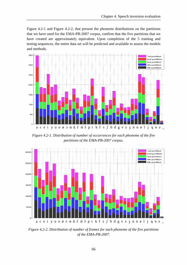
Chapter 4. Speech inversion evaluation
66
Figure 4.2-1 and Figure 4.2-2, that present the phoneme distributions on the partitions that we have used for the EMA-PB-2007 corpus, confirm that the five partitions that we have created are approximately equivalent. Upon completion of the 5 training and testing sequences, the entire data set will be predicted and available to assess the models and methods.
a ɛ e i y u o ø ɔ œɑ̃ ɛ ̃ œ̃ɔ̃ p t k f s ʃ b d g v z ʒ m n ʁ l j ɥ w ə _
Figure 4.2-1. Distribution of number of occurrences for each phoneme of the five partitions of the EMA-PB-2007 corpus.
a ɛ e i y u o ø ɔ œɑ̃ ɛ ̃ œ̃ɔ̃ p t k f s ʃ b d g v z ʒ m n ʁ l j ɥ w ə _
Figure 4.2-2. Distribution of number of frames for each phoneme of the five partitions of the EMA-PB-2007.

Chapter 4. Speech inversion evaluation
67
4.2.2. Measurements
The Root Mean Square Error (RMSE) and the Pearson Product-Moment Correlation Coefficient (PMCC), between the measured and estimated date, are usually used in the literature to evaluate inversion systems. We have also used these two criteria and calculated them over the five test partitions – therefore the whole corpus –, excluding the long pauses at the beginning and the end of each utterance.
For each EMA coordinate, we calculated the RMSEd between the measured and the estimated trajectory as:
( )2
, ,1
1ˆ
T
d d t d tt
RMSE y yT =
= −∑ (4.2-1)
where T is the number of frames aggregated over the five partitions of the test set, and
,ˆ
d ty and
,d ty are respectively the estimated and the measured values of the dth EMA
coordinate at time t.
The global accuracy of the inversion was measured in different ways.
We calculated two global RMSE over all coordinates. The first was:
( )2
1
1 D
dd
RMSE RMSED =
= ∑ (4.2-2)
where D is the number of EMA coordinates.
We calculated also the slightly different – producing an error mathematically always inferior to the preceding formula – formulation of the global RMSE often found in the literature (as in (Hiroya and Honda, 2004), (Zhang and Renals, 2008), (Ling et al., 2010) or (Toda et al., 2008)). This RMSE, called here µRMSE, is averaged over all coordinates as:
1
1 D
dd
RMSE RMSED
µ=
= ∑ (4.2-3)
We also calculated the “Pearson Product-Moment Correlation Coefficient” (PMCC) which measures the level of amplitude similarity and synchrony of the trajectories as
( )( )
( ) ( )
, ,1 1
2 2
, ,1 1 1 1
ˆ ˆ
ˆ ˆ
D T
d t d d t dd t
D T D T
d t d d t dd t d t
y y y yPPMC
y y y y
= =
= = = =
− −=
− −
∑∑
∑∑ ∑∑
(4.2-4)
Chapter 4. Speech inversion evaluation
68
Where ˆdy and dy represent the mean values of the estimated and measured trajectories
of the dth EMA coordinate.
4.2.3. Acoustic recognition
The HMM-based inversion method involves an intermediary stage of automatic recognition. The acoustic recognition accuracy (Acc) is also aggregated, over the five partitions of the test set, to assess specifically the associated acoustic phonetic decoding stage and is defined as:
100%N D S I
AccN
− − −= × (4.2-5)
where N, S, D and I are the total number of phones, the number of substitution errors, the number of deletion errors, and the number of insertion errors respectively. The acoustic recognition correct (Correct) that ignores insertion errors was defined as
Correct 100%
N D S
N
− −= × (4.2-6)
4.2.4. Articulatory spaces
Another interesting way to analyse the performance of an inversion method is to compare visually, for the measured and reconstructed data, the articulatory spaces of the EMA coils, i.e. the spaces in the midsagittal plane covered by the six coils for the whole corpuses (cf. further Figure 4.3-1). This could be complemented by a measure of the degree of overlap between the areas of measured and estimated articulatory spaces.
4.2.5. Articulatory recognition
4.2.5.1 Method
When original articulatory data are not available, in particular in the case of inversion of a new speaker, using an acoustic adaptation stage (see Chapter 5), the RMSE criterium cannot be used. In such a case, an interesting alternative way to evaluate estimated articulatory trajectories is to determine how well they can be recognised by an automatic “articulatory recognition” system trained on the original data. Engwall (2006) proposes an articulatory classifier to evaluate the results of speech inversion. In addition to the correlation coefficients and the RMS error, he presents classification scores summarized as the percentage of correctly classified phonemes and places of articulation, as the performance for different phoneme groups and in confusion matrices. Tepperman et al. (2008) presents hidden articulator Markov models, which were trained on articulatory representation of phone-level transcription, to generate articulatory confidence measures and recognition-based feature. With this purpose, we
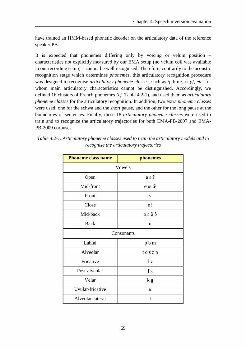
Chapter 4. Speech inversion evaluation
69
have trained an HMM-based phonetic decoder on the articulatory data of the reference speaker PB.
It is expected that phonemes differing only by voicing or velum position – characteristics not explicitly measured by our EMA setup (no velum coil was available in our recording setup) – cannot be well recognised. Therefore, contrarily to the acoustic recognition stage which determines phonemes, this articulatory recognition procedure was designed to recognise articulatory phoneme classes, such as /p b m/, /k g/, etc. for whom main articulatory characteristics cannot be distinguished. Accordingly, we defined 16 clusters of French phonemes (cf. Table 4.2-1), and used them as articulatory phoneme classes for the articulatory recognition. In addition, two extra phoneme classes were used: one for the schwa and the short pause, and the other for the long pause at the boundaries of sentences. Finally, these 18 articulatory phoneme classes were used to train and to recognize the articulatory trajectories for both EMA-PB-2007 and EMA-PB-2009 corpuses.
Table 4.2-1. Articulatory phoneme classes used to train the articulatory models and to recognise the articulatory trajectories
Phoneme class name phonemes
Vowels
Open a ɛ ɛ ̃
Mid-front ø œ œ̃
Front y
Close e i
Mid-back o ɔ ɑ̃ ɔ̃
Back u
Consonants
Labial p b m
Alveolar t d s z n
Fricative f v
Post-alveolar ʃ ʒ
Velar k g
Uvular-fricative ʁ
Alveolar-lateral l
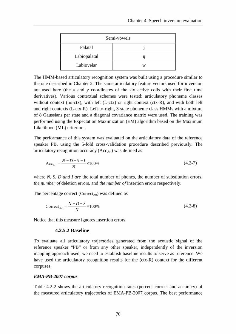
Chapter 4. Speech inversion evaluation
70
Semi-vowels
Palatal j
Labiopalatal ɥ
Labiovelar w
The HMM-based articulatory recognition system was built using a procedure similar to the one described in Chapter 2. The same articulatory feature vectors used for inversion are used here (the x and y coordinates of the six active coils with their first time derivatives). Various contextual schemes were tested: articulatory phoneme classes without context (no-ctx), with left (L-ctx) or right context (ctx-R), and with both left and right contexts (L-ctx-R). Left-to-right, 3-state phoneme class HMMs with a mixture of 8 Gaussians per state and a diagonal covariance matrix were used. The training was performed using the Expectation Maximization (EM) algorithm based on the Maximum Likelihood (ML) criterion.
The performance of this system was evaluated on the articulatory data of the reference speaker PB, using the 5-fold cross-validation procedure described previously. The articulatory recognition accuracy (AccArt) was defined as
ArtAcc 100%
N D S I
N
− − −= × (4.2-7)
where N, S, D and I are the total number of phones, the number of substitution errors, the number of deletion errors, and the number of insertion errors respectively.
The percentage correct (CorrectArt) was defined as
ArtCorrect 100%
N D S
N
− −= × (4.2-8)
Notice that this measure ignores insertion errors.
4.2.5.2 Baseline
To evaluate all articulatory trajectories generated from the acoustic signal of the reference speaker “PB” or from any other speaker, independently of the inversion mapping approach used, we need to establish baseline results to serve as reference. We have used the articulatory recognition results for the (ctx-R) context for the different corpuses.
EMA-PB-2007 corpus
Table 4.2-2 shows the articulatory recognition rates (percent correct and accuracy) of the measured articulatory trajectories of EMA-PB-2007 corpus. The best performance
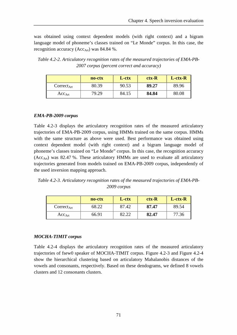
Chapter 4. Speech inversion evaluation
71
was obtained using context dependent models (with right context) and a bigram language model of phoneme’s classes trained on “Le Monde” corpus. In this case, the recognition accuracy (AccArt) was 84.84 %.
Table 4.2-2. Articulatory recognition rates of the measured trajectories of EMA-PB-2007 corpus (percent correct and accuracy)
no-ctx L-ctx ctx-R L-ctx-R
CorrectArt 80.39 90.53 89.27 89.96
AccArt 79.29 84.15 84.84 80.08
EMA-PB-2009 corpus
Table 4.2-3 displays the articulatory recognition rates of the measured articulatory trajectories of EMA-PB-2009 corpus, using HMMs trained on the same corpus. HMMs with the same structure as above were used. Best performance was obtained using context dependent model (with right context) and a bigram language model of phoneme’s classes trained on “Le Monde” corpus. In this case, the recognition accuracy (AccArt) was 82.47 %. These articulatory HMMs are used to evaluate all articulatory trajectories generated from models trained on EMA-PB-2009 corpus, independently of the used inversion mapping approach.
Table 4.2-3. Articulatory recognition rates of the measured trajectories of EMA-PB-2009 corpus
no-ctx L-ctx ctx-R L-ctx-R
CorrectArt 68.22 87.42 87.47 89.54
AccArt 66.91 82.22 82.47 77.36
MOCHA-TIMIT corpus
Table 4.2-4 displays the articulatory recognition rates of the measured articulatory trajectories of fsew0 speaker of MOCHA-TIMIT corpus. Figure 4.2-3 and Figure 4.2-4 show the hierarchical clustering based on articulatory Mahalanobis distances of the vowels and consonants, respectively. Based on these dendograms, we defined 8 vowels clusters and 12 consonants clusters.
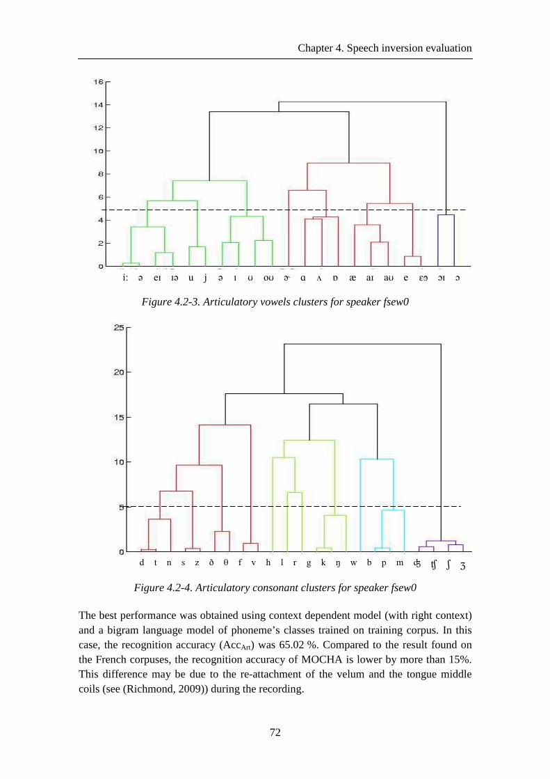
Chapter 4. Speech inversion evaluation
72
i: ə eɪ ɪə u j ə ɪ ʊ oʊ ɚ ɑ ʌ ɒ æ aɪ aʊ e ɛɘ ɔɪ ɔ
Figure 4.2-3. Articulatory vowels clusters for speaker fsew0
d t n s z ð θ f v h l r g k ŋ w b p m ʤ ʧ ʃ ʒ
Figure 4.2-4. Articulatory consonant clusters for speaker fsew0
The best performance was obtained using context dependent model (with right context) and a bigram language model of phoneme’s classes trained on training corpus. In this case, the recognition accuracy (AccArt) was 65.02 %. Compared to the result found on the French corpuses, the recognition accuracy of MOCHA is lower by more than 15%. This difference may be due to the re-attachment of the velum and the tongue middle coils (see (Richmond, 2009)) during the recording.
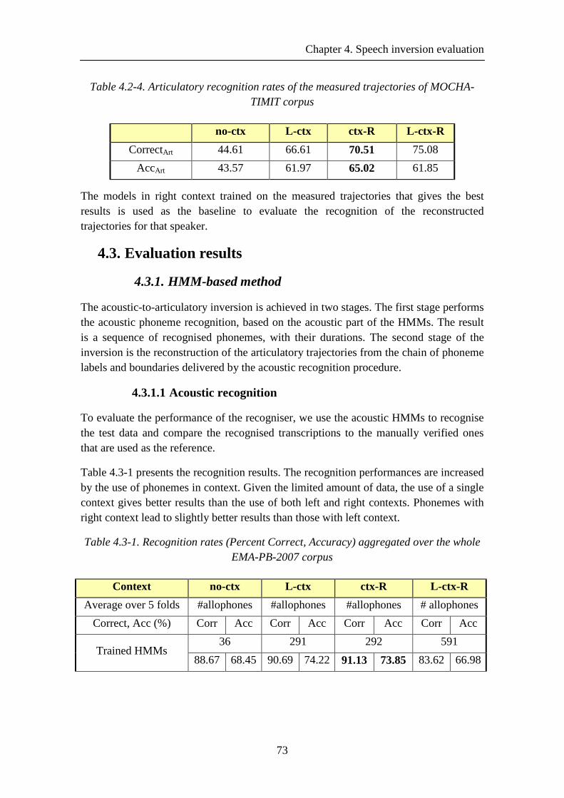
Chapter 4. Speech inversion evaluation
73
Table 4.2-4. Articulatory recognition rates of the measured trajectories of MOCHA-TIMIT corpus
no-ctx L-ctx ctx-R L-ctx-R
CorrectArt 44.61 66.61 70.51 75.08
AccArt 43.57 61.97 65.02 61.85
The models in right context trained on the measured trajectories that gives the best results is used as the baseline to evaluate the recognition of the reconstructed trajectories for that speaker.
4.3. Evaluation results
4.3.1. HMM-based method
The acoustic-to-articulatory inversion is achieved in two stages. The first stage performs the acoustic phoneme recognition, based on the acoustic part of the HMMs. The result is a sequence of recognised phonemes, with their durations. The second stage of the inversion is the reconstruction of the articulatory trajectories from the chain of phoneme labels and boundaries delivered by the acoustic recognition procedure.
4.3.1.1 Acoustic recognition
To evaluate the performance of the recogniser, we use the acoustic HMMs to recognise the test data and compare the recognised transcriptions to the manually verified ones that are used as the reference.
Table 4.3-1 presents the recognition results. The recognition performances are increased by the use of phonemes in context. Given the limited amount of data, the use of a single context gives better results than the use of both left and right contexts. Phonemes with right context lead to slightly better results than those with left context.
Table 4.3-1. Recognition rates (Percent Correct, Accuracy) aggregated over the whole EMA-PB-2007 corpus
Context no-ctx L-ctx ctx-R L-ctx-R
Average over 5 folds #allophones #allophones #allophones # allophones
Correct, Acc (%) Corr Acc Corr Acc Corr Acc Corr Acc
Trained HMMs 36 291 292 591
88.67 68.45 90.69 74.22 91.13 73.85 83.62 66.98
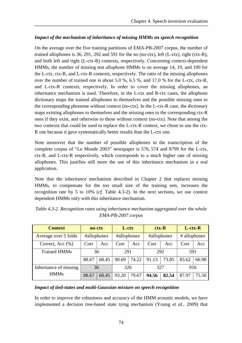
Chapter 4. Speech inversion evaluation
74
Impact of the mechanism of inheritance of missing HMMs on speech recognition
On the average over the five training partitions of EMA-PB-2007 corpus, the number of trained allophones is 36, 291, 292 and 591 for the no (no-ctx), left (L-ctx), right (ctx-R), and both left and right (L-ctx-R) contexts, respectively. Concerning context-dependent HMMs, the number of missing test allophone HMMs is on average 14, 19, and 100 for the L-ctx, ctx-R, and L-ctx-R contexts, respectively. The ratio of the missing allophones over the number of trained one is about 5.0 %, 6.5 %, and 17.0 % for the L-ctx, ctx-R, and L-ctx-R contexts, respectively. In order to cover the missing allophones, an inheritance mechanism is used. Therefore, in the L-ctx and R-ctx cases, the allophone dictionary maps the trained allophones to themselves and the possible missing ones to the corresponding phoneme without context (no-ctx). In the L-ctx-R case, the dictionary maps existing allophones to themselves and the missing ones to the corresponding ctx-R ones if they exist, and otherwise to those without context (no-ctx). Note that among the two contexts that could be used to replace the L-ctx-R context, we chose to use the ctx-R one because it gave systematically better results than the L-ctx one.
Note moreover that the number of possible allophones in the transcription of the complete corpus of “Le Monde 2003” newspaper is 576, 574 and 8799 for the L-ctx, ctx-R, and L-ctx-R respectively, which corresponds to a much higher rate of missing allophones. This justifies still more the use of this inheritance mechanism in a real application.
Note that the inheritance mechanism described in Chapter 2 that replaces missing HMMs, to compensate for the too small size of the training sets, increases the recognition rate by 5 to 10% (cf. Table 4.3-2). In the next sections, we use context dependent HMMs only with this inheritance mechanism.
Table 4.3-2. Recognition rates using inheritance mechanism aggregated over the whole EMA-PB-2007 corpus
Context no-ctx L-ctx ctx-R L-ctx-R
Average over 5 folds #allophones #allophones #allophones # allophones
Correct, Acc (%) Corr Acc Corr Acc Corr Acc Corr Acc
Trained HMMs 36 291 292 591
88.67 68.45 90.69 74.22 91.13 73.85 83.62 66.98
Inheritance of missing HMMs
36 326 327 916
88.67 68.45 93.20 79.67 94.56 82.54 87.97 75.50
Impact of tied-states and multi-Gaussian mixture on speech recognition
In order to improve the robustness and accuracy of the HMM acoustic models, we have implemented a decision tree-based state tying mechanism (Young et al., 2009) that
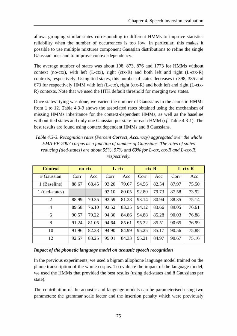
Chapter 4. Speech inversion evaluation
75
allows grouping similar states corresponding to different HMMs to improve statistics reliability when the number of occurrences is too low. In particular, this makes it possible to use multiple mixtures component Gaussian distributions to refine the single Gaussian ones and to improve context-dependency.
The average number of states was about 108, 873, 876 and 1773 for HMMs without context (no-ctx), with left (L-ctx), right (ctx-R) and both left and right (L-ctx-R) contexts, respectively. Using tied states, this number of states decreases to 398, 385 and 673 for respectively HMM with left (L-ctx), right (ctx-R) and both left and right (L-ctx-R) contexts. Note that we used the HTK default threshold for merging two states.
Once states’ tying was done, we varied the number of Gaussians in the acoustic HMMs from 1 to 12. Table 4.3-3 shows the associated rates obtained using the mechanism of missing HMMs inheritance for the context-dependent HMMs, as well as the baseline without tied states and only one Gaussian per state for each HMM (cf. Table 4.3-1). The best results are found using context dependent HMMs and 8 Gaussians.
Table 4.3-3. Recognition rates (Percent Correct, Accuracy) aggregated over the whole EMA-PB-2007 corpus as a function of number of Gaussians. The rates of states
reducing (tied-states) are about 55%, 57% and 63% for L-ctx, ctx-R and L-ctx-R, respectively.
Context no-ctx L-ctx ctx-R L-ctx-R
# Gaussian Corr Acc Corr Acc Corr Acc Corr Acc
1 (Baseline) 88.67 68.45 93.20 79.67 94.56 82.54 87.97 75.50
1 (tied-states) 92.10 80.05 92.80 79.73 87.58 73.92
2 88.99 70.35 92.59 81.28 93.14 80.94 88.35 75.14
4 89.58 76.10 93.52 83.35 94.12 83.66 89.05 76.61
6 90.57 79.22 94.30 84.86 94.88 85.28 90.03 76.88
8 91.24 81.05 94.64 85.61 95.22 85.51 90.65 76.99
10 91.96 82.33 94.90 84.99 95.25 85.17 90.56 75.88
12 92.57 83.25 95.01 84.33 95.21 84.97 90.67 75.16
Impact of the phonetic language model on acoustic speech recognition
In the previous experiments, we used a bigram allophone language model trained on the phone transcription of the whole corpus. To evaluate the impact of the language model, we used the HMMs that provided the best results (using tied-states and 8 Gaussians per state).
The contribution of the acoustic and language models can be parameterised using two parameters: the grammar scale factor and the insertion penalty which were previously
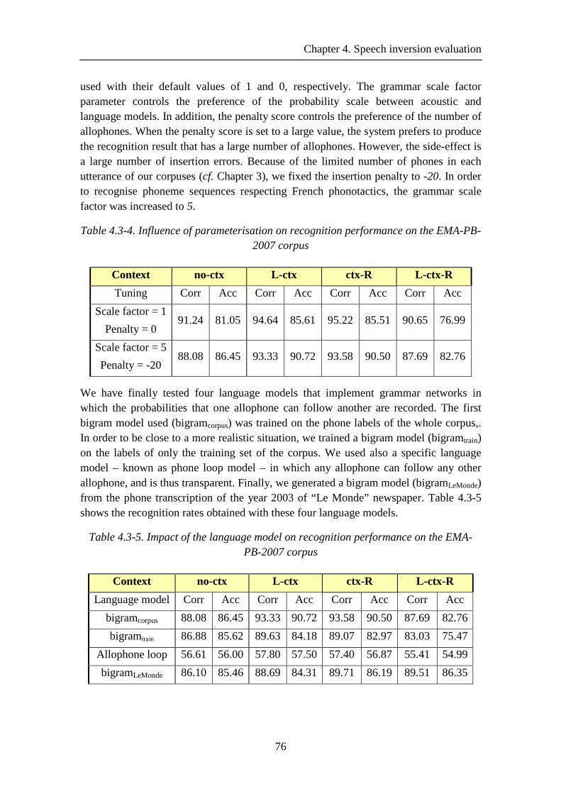
Chapter 4. Speech inversion evaluation
76
used with their default values of 1 and 0, respectively. The grammar scale factor parameter controls the preference of the probability scale between acoustic and language models. In addition, the penalty score controls the preference of the number of allophones. When the penalty score is set to a large value, the system prefers to produce the recognition result that has a large number of allophones. However, the side-effect is a large number of insertion errors. Because of the limited number of phones in each utterance of our corpuses (cf. Chapter 3), we fixed the insertion penalty to -20. In order to recognise phoneme sequences respecting French phonotactics, the grammar scale factor was increased to 5.
Table 4.3-4. Influence of parameterisation on recognition performance on the EMA-PB-2007 corpus
Context no-ctx L-ctx ctx-R L-ctx-R
Tuning Corr Acc Corr Acc Corr Acc Corr Acc
Scale factor = 1
Penalty = 0 91.24 81.05 94.64 85.61 95.22 85.51 90.65 76.99
Scale factor = 5
Penalty = -20 88.08 86.45 93.33 90.72 93.58 90.50 87.69 82.76
We have finally tested four language models that implement grammar networks in which the probabilities that one allophone can follow another are recorded. The first bigram model used (bigramcorpus) was trained on the phone labels of the whole corpus,. In order to be close to a more realistic situation, we trained a bigram model (bigramtrain) on the labels of only the training set of the corpus. We used also a specific language model – known as phone loop model – in which any allophone can follow any other allophone, and is thus transparent. Finally, we generated a bigram model (bigramLeMonde) from the phone transcription of the year 2003 of “Le Monde” newspaper. Table 4.3-5 shows the recognition rates obtained with these four language models.
Table 4.3-5. Impact of the language model on recognition performance on the EMA-PB-2007 corpus
Context no-ctx L-ctx ctx-R L-ctx-R
Language model Corr Acc Corr Acc Corr Acc Corr Acc
bigramcorpus 88.08 86.45 93.33 90.72 93.58 90.50 87.69 82.76
bigramtrain 86.88 85.62 89.63 84.18 89.07 82.97 83.03 75.47
Allophone loop 56.61 56.00 57.80 57.50 57.40 56.87 55.41 54.99
bigramLeMonde 86.10 85.46 88.69 84.31 89.71 86.19 89.51 86.35
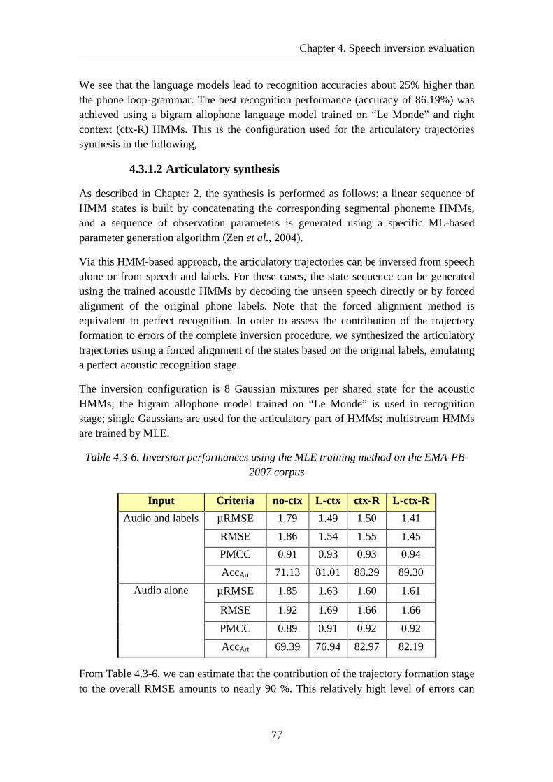
Chapter 4. Speech inversion evaluation
77
We see that the language models lead to recognition accuracies about 25% higher than the phone loop-grammar. The best recognition performance (accuracy of 86.19%) was achieved using a bigram allophone language model trained on “Le Monde” and right context (ctx-R) HMMs. This is the configuration used for the articulatory trajectories synthesis in the following,
4.3.1.2 Articulatory synthesis
As described in Chapter 2, the synthesis is performed as follows: a linear sequence of HMM states is built by concatenating the corresponding segmental phoneme HMMs, and a sequence of observation parameters is generated using a specific ML-based parameter generation algorithm (Zen et al., 2004).
Via this HMM-based approach, the articulatory trajectories can be inversed from speech alone or from speech and labels. For these cases, the state sequence can be generated using the trained acoustic HMMs by decoding the unseen speech directly or by forced alignment of the original phone labels. Note that the forced alignment method is equivalent to perfect recognition. In order to assess the contribution of the trajectory formation to errors of the complete inversion procedure, we synthesized the articulatory trajectories using a forced alignment of the states based on the original labels, emulating a perfect acoustic recognition stage.
The inversion configuration is 8 Gaussian mixtures per shared state for the acoustic HMMs; the bigram allophone model trained on “Le Monde” is used in recognition stage; single Gaussians are used for the articulatory part of HMMs; multistream HMMs are trained by MLE.
Table 4.3-6. Inversion performances using the MLE training method on the EMA-PB-2007 corpus
Input Criteria no-ctx L-ctx ctx-R L-ctx-R
Audio and labels µRMSE 1.79 1.49 1.50 1.41
RMSE 1.86 1.54 1.55 1.45
PMCC 0.91 0.93 0.93 0.94
AccArt 71.13 81.01 88.29 89.30
Audio alone µRMSE 1.85 1.63 1.60 1.61
RMSE 1.92 1.69 1.66 1.66
PMCC 0.89 0.91 0.92 0.92
AccArt 69.39 76.94 82.97 82.19
From Table 4.3-6, we can estimate that the contribution of the trajectory formation stage to the overall RMSE amounts to nearly 90 %. This relatively high level of errors can
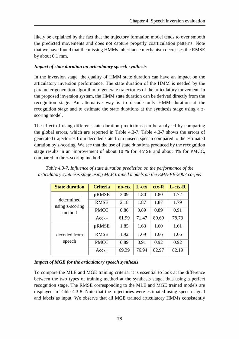
Chapter 4. Speech inversion evaluation
78
likely be explained by the fact that the trajectory formation model tends to over smooth the predicted movements and does not capture properly coarticulation patterns. Note that we have found that the missing HMMs inheritance mechanism decreases the RMSE by about 0.1 mm.
Impact of state duration on articulatory speech synthesis
In the inversion stage, the quality of HMM state duration can have an impact on the articulatory inversion performance. The state duration of the HMM is needed by the parameter generation algorithm to generate trajectories of the articulatory movement. In the proposed inversion system, the HMM state duration can be derived directly from the recognition stage. An alternative way is to decode only HMM duration at the recognition stage and to estimate the state durations at the synthesis stage using a z-scoring model.
The effect of using different state duration predictions can be analysed by comparing the global errors, which are reported in Table 4.3-7. Table 4.3-7 shows the errors of generated trajectories from decoded state from unseen speech compared to the estimated duration by z-scoring. We see that the use of state durations produced by the recognition stage results in an improvement of about 10 % for RMSE and about 4% for PMCC, compared to the z-scoring method.
Table 4.3-7. Influence of state duration prediction on the performance of the articulatory synthesis stage using MLE trained models on the EMA-PB-2007 corpus
State duration Criteria no-ctx L-ctx ctx-R L-ctx-R
determined using z-scoring
method
µRMSE 2.09 1.80 1.80 1.72
RMSE 2,18 1.87 1,87 1.79
PMCC 0,86 0,89 0,89 0,91
AccArt 61.99 71.47 80.60 78.73
decoded from speech
µRMSE 1.85 1.63 1.60 1.61
RMSE 1.92 1.69 1.66 1.66
PMCC 0.89 0.91 0.92 0.92
AccArt 69.39 76.94 82.97 82.19
Impact of MGE for the articulatory speech synthesis
To compare the MLE and MGE training criteria, it is essential to look at the difference between the two types of training method at the synthesis stage, thus using a perfect recognition stage. The RMSE corresponding to the MLE and MGE trained models are displayed in Table 4.3-8. Note that the trajectories were estimated using speech signal and labels as input. We observe that all MGE trained articulatory HMMs consistently
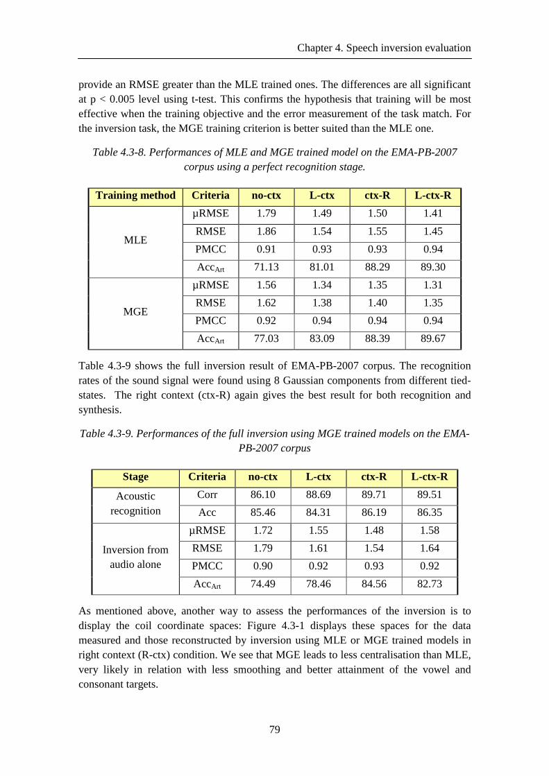
Chapter 4. Speech inversion evaluation
79
provide an RMSE greater than the MLE trained ones. The differences are all significant at p < 0.005 level using t-test. This confirms the hypothesis that training will be most effective when the training objective and the error measurement of the task match. For the inversion task, the MGE training criterion is better suited than the MLE one.
Table 4.3-8. Performances of MLE and MGE trained model on the EMA-PB-2007 corpus using a perfect recognition stage.
Training method Criteria no-ctx L-ctx ctx-R L-ctx-R
MLE
µRMSE 1.79 1.49 1.50 1.41
RMSE 1.86 1.54 1.55 1.45
PMCC 0.91 0.93 0.93 0.94
AccArt 71.13 81.01 88.29 89.30
MGE
µRMSE 1.56 1.34 1.35 1.31
RMSE 1.62 1.38 1.40 1.35
PMCC 0.92 0.94 0.94 0.94
AccArt 77.03 83.09 88.39 89.67
Table 4.3-9 shows the full inversion result of EMA-PB-2007 corpus. The recognition rates of the sound signal were found using 8 Gaussian components from different tied-states. The right context (ctx-R) again gives the best result for both recognition and synthesis.
Table 4.3-9. Performances of the full inversion using MGE trained models on the EMA-PB-2007 corpus
Stage Criteria no-ctx L-ctx ctx-R L-ctx-R
Acoustic recognition
Corr 86.10 88.69 89.71 89.51
Acc 85.46 84.31 86.19 86.35
Inversion from audio alone
µRMSE 1.72 1.55 1.48 1.58
RMSE 1.79 1.61 1.54 1.64
PMCC 0.90 0.92 0.93 0.92
AccArt 74.49 78.46 84.56 82.73
As mentioned above, another way to assess the performances of the inversion is to display the coil coordinate spaces: Figure 4.3-1 displays these spaces for the data measured and those reconstructed by inversion using MLE or MGE trained models in right context (R-ctx) condition. We see that MGE leads to less centralisation than MLE, very likely in relation with less smoothing and better attainment of the vowel and consonant targets.
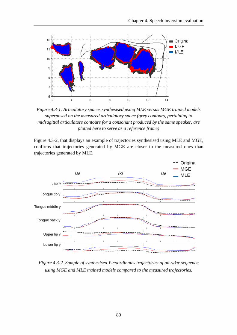
Chapter 4. Speech inversion evaluation
80
Figure 4.3-1. Articulatory spaces synthesised using MLE versus MGE trained models superposed on the measured articulatory space (grey contours, pertaining to
midsagittal articulators contours for a consonant produced by the same speaker, are plotted here to serve as a reference frame)
Figure 4.3-2, that displays an example of trajectories synthesised using MLE and MGE, confirms that trajectories generated by MGE are closer to the measured ones than trajectories generated by MLE.
Tongue tip y
Tongue middle y
Tongue back y
OriginalMGEMLE /a/ /k/ /a/
Jaw y
Upper lip y
Lower lip y
Figure 4.3-2. Sample of synthesised Y-coordinates trajectories of an /aka/ sequence
using MGE and MLE trained models compared to the measured trajectories.
Chapter 4. Speech inversion evaluation
81
4.3.1.3 HMM-based results
In order to assess the influence of the corpus on the inversion performances, we analyse in this section the inversion results obtained on two other corpuses: EMA-PB-2009 and MOCHA-TIMIT speaker fsew0.
The same improvement described above was applied to these corpuses. We varied the number of Gaussians for the acoustic HMMs. For the articulatory HMMs, using more than one Gaussian did not improve the results, and therefore only one Gaussian was used. Therefore, we used the MGE training criterion to improve the articulatory models. Table 4.3-10, which displays the inversion results, using 8 Gaussians for the acoustic HMMs, the RMSE and correlation coefficients for the HMM-based inversion, shows that the use of phones in context increases the performance of the inversion. The EMA-PB-2009 corpus contains more data than the EMA-PB-2007 one. But the best results are however not obtained for the phones with both right and left contexts, but for the phones with the right context.
Using a language model trained on “Le Monde” corpus, we found an acoustic recognition accuracy of 84.00 % for the phone in right context case. This rate gives an RMSE of 1.45 mm and a correlation coefficient of 0.90.
Besides, to assess the contribution of the trajectory formation to errors of the complete inversion procedure, we also synthesized these trajectories using a forced alignment of the states based on the original labels, emulating a perfect acoustic recognition stage. Table 4.3-10, we can estimate that the contribution of the trajectory formation stage to the overall RMSE amounts to nearly 90 %. This relatively high level of errors can likely be explained by the fact that the trajectory formation model tends to over-smooth the predicted movements and does not capture properly coarticulation patterns.
In order to compare our method to the literature, we applied the improvement of the acoustic and articulatory HMMs jointly initialised on the MOCHA-TIMIT corpus. As for the French corpuses, we found using a language model trained on the labels on the training corpus, 8 Gaussians on the acoustic HMMs and MGE trained articulatory HMMs that the right context (ctx-R) gave the best result. Section 4.4 presents the comparisons.
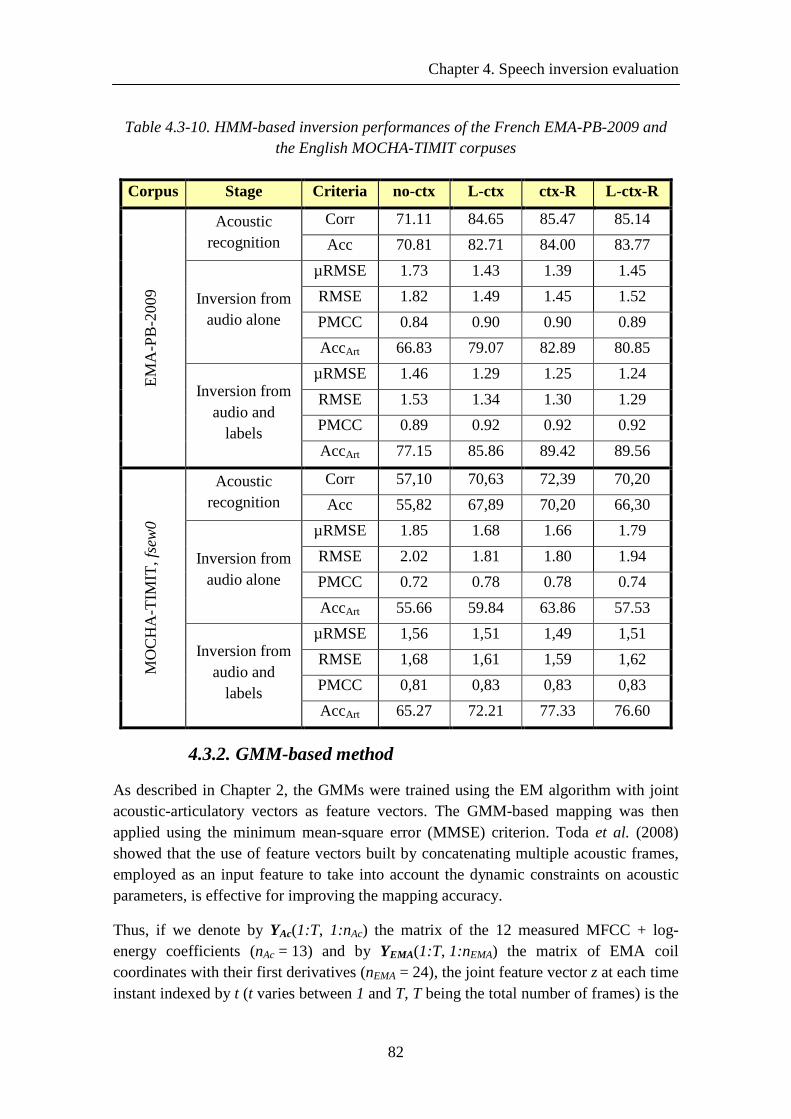
Chapter 4. Speech inversion evaluation
82
Table 4.3-10. HMM-based inversion performances of the French EMA-PB-2009 and the English MOCHA-TIMIT corpuses
Corpus Stage Criteria no-ctx L-ctx ctx-R L-ctx-R
EM
A-P
B-2
009
Acoustic recognition
Corr 71.11 84.65 85.47 85.14
Acc 70.81 82.71 84.00 83.77
Inversion from audio alone
µRMSE 1.73 1.43 1.39 1.45
RMSE 1.82 1.49 1.45 1.52
PMCC 0.84 0.90 0.90 0.89
AccArt 66.83 79.07 82.89 80.85
Inversion from audio and
labels
µRMSE 1.46 1.29 1.25 1.24
RMSE 1.53 1.34 1.30 1.29
PMCC 0.89 0.92 0.92 0.92
AccArt 77.15 85.86 89.42 89.56
MO
CH
A-T
IMIT
, fs
ew
0
Acoustic recognition
Corr 57,10 70,63 72,39 70,20
Acc 55,82 67,89 70,20 66,30
Inversion from audio alone
µRMSE 1.85 1.68 1.66 1.79
RMSE 2.02 1.81 1.80 1.94
PMCC 0.72 0.78 0.78 0.74
AccArt 55.66 59.84 63.86 57.53
Inversion from audio and
labels
µRMSE 1,56 1,51 1,49 1,51
RMSE 1,68 1,61 1,59 1,62
PMCC 0,81 0,83 0,83 0,83
AccArt 65.27 72.21 77.33 76.60
4.3.2. GMM-based method
As described in Chapter 2, the GMMs were trained using the EM algorithm with joint acoustic-articulatory vectors as feature vectors. The GMM-based mapping was then applied using the minimum mean-square error (MMSE) criterion. Toda et al. (2008) showed that the use of feature vectors built by concatenating multiple acoustic frames, employed as an input feature to take into account the dynamic constraints on acoustic parameters, is effective for improving the mapping accuracy.
Thus, if we denote by YAc(1:T, 1:nAc) the matrix of the 12 measured MFCC + log-energy coefficients (nAc = 13) and by YEMA(1:T, 1:nEMA) the matrix of EMA coil coordinates with their first derivatives (nEMA = 24), the joint feature vector z at each time instant indexed by t (t varies between 1 and T, T being the total number of frames) is the
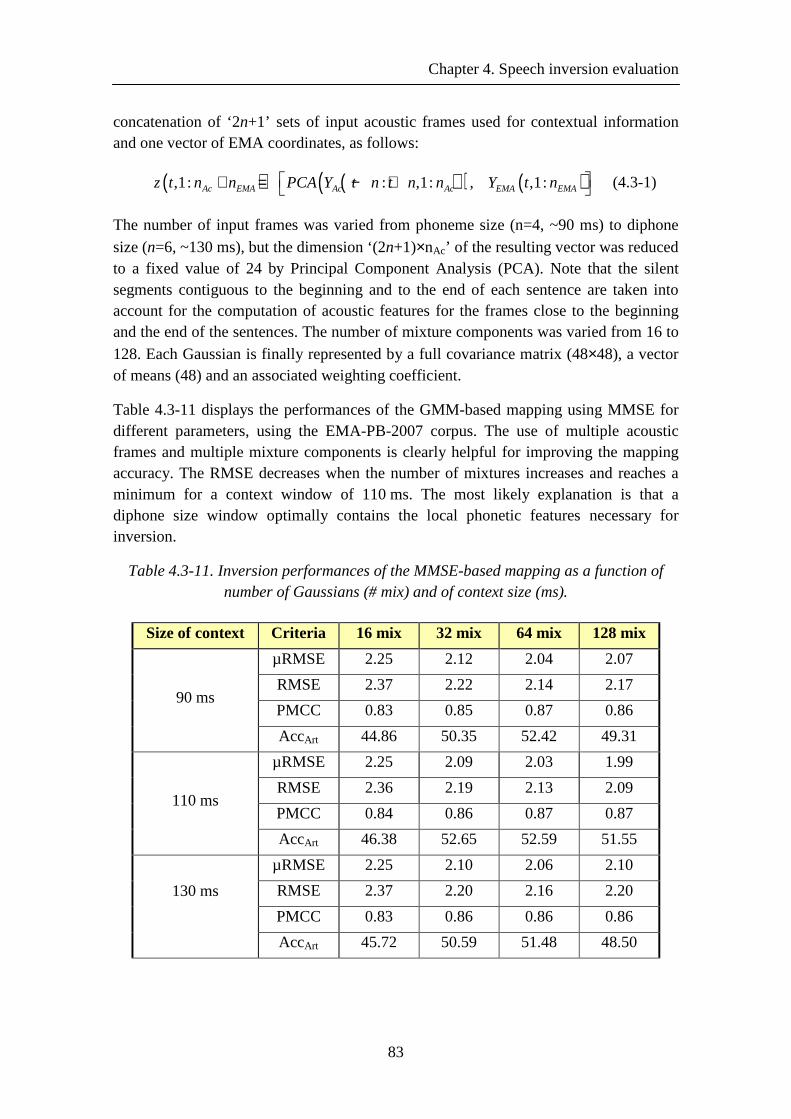
Chapter 4. Speech inversion evaluation
83
concatenation of ‘2n+1’ sets of input acoustic frames used for contextual information and one vector of EMA coordinates, as follows:
( ) ( )( ) ( ),1: : ,1: , ,1:Ac EMA Ac Ac EMA EMAz t n n PCA Y t n t n n Y t n + = − + (4.3-1)
The number of input frames was varied from phoneme size (n=4, ~90 ms) to diphone size (n=6, ~130 ms), but the dimension ‘(2n+1)×nAc’ of the resulting vector was reduced to a fixed value of 24 by Principal Component Analysis (PCA). Note that the silent segments contiguous to the beginning and to the end of each sentence are taken into account for the computation of acoustic features for the frames close to the beginning and the end of the sentences. The number of mixture components was varied from 16 to 128. Each Gaussian is finally represented by a full covariance matrix (48×48), a vector of means (48) and an associated weighting coefficient.
Table 4.3-11 displays the performances of the GMM-based mapping using MMSE for different parameters, using the EMA-PB-2007 corpus. The use of multiple acoustic frames and multiple mixture components is clearly helpful for improving the mapping accuracy. The RMSE decreases when the number of mixtures increases and reaches a minimum for a context window of 110 ms. The most likely explanation is that a diphone size window optimally contains the local phonetic features necessary for inversion.
Table 4.3-11. Inversion performances of the MMSE-based mapping as a function of number of Gaussians (# mix) and of context size (ms).
Size of context Criteria 16 mix 32 mix 64 mix 128 mix
90 ms
µRMSE 2.25 2.12 2.04 2.07
RMSE 2.37 2.22 2.14 2.17
PMCC 0.83 0.85 0.87 0.86
AccArt 44.86 50.35 52.42 49.31
110 ms
µRMSE 2.25 2.09 2.03 1.99
RMSE 2.36 2.19 2.13 2.09
PMCC 0.84 0.86 0.87 0.87
AccArt 46.38 52.65 52.59 51.55
130 ms
µRMSE 2.25 2.10 2.06 2.10
RMSE 2.37 2.20 2.16 2.20
PMCC 0.83 0.86 0.86 0.86
AccArt 45.72 50.59 51.48 48.50
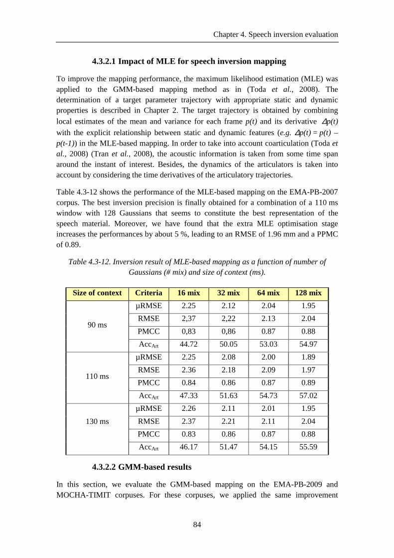
Chapter 4. Speech inversion evaluation
84
4.3.2.1 Impact of MLE for speech inversion mapping
To improve the mapping performance, the maximum likelihood estimation (MLE) was applied to the GMM-based mapping method as in (Toda et al., 2008). The determination of a target parameter trajectory with appropriate static and dynamic properties is described in Chapter 2. The target trajectory is obtained by combining local estimates of the mean and variance for each frame p(t) and its derivative ∆p(t)
with the explicit relationship between static and dynamic features (e.g. ∆p(t) = p(t) – p(t-1)) in the MLE-based mapping. In order to take into account coarticulation (Toda et al., 2008) (Tran et al., 2008), the acoustic information is taken from some time span around the instant of interest. Besides, the dynamics of the articulators is taken into account by considering the time derivatives of the articulatory trajectories.
Table 4.3-12 shows the performance of the MLE-based mapping on the EMA-PB-2007 corpus. The best inversion precision is finally obtained for a combination of a 110 ms window with 128 Gaussians that seems to constitute the best representation of the speech material. Moreover, we have found that the extra MLE optimisation stage increases the performances by about 5 %, leading to an RMSE of 1.96 mm and a PPMC of 0.89.
Table 4.3-12. Inversion result of MLE-based mapping as a function of number of Gaussians (# mix) and size of context (ms).
Size of context Criteria 16 mix 32 mix 64 mix 128 mix
90 ms
µRMSE 2.25 2.12 2.04 1.95
RMSE 2,37 2,22 2.13 2.04
PMCC 0,83 0,86 0.87 0.88
AccArt 44.72 50.05 53.03 54.97
110 ms
µRMSE 2.25 2.08 2.00 1.89
RMSE 2.36 2.18 2.09 1.97
PMCC 0.84 0.86 0.87 0.89
AccArt 47.33 51.63 54.73 57.02
130 ms
µRMSE 2.26 2.11 2.01 1.95
RMSE 2.37 2.21 2.11 2.04
PMCC 0.83 0.86 0.87 0.88
AccArt 46.17 51.47 54.15 55.59
4.3.2.2 GMM-based results
In this section, we evaluate the GMM-based mapping on the EMA-PB-2009 and MOCHA-TIMIT corpuses. For these corpuses, we applied the same improvement
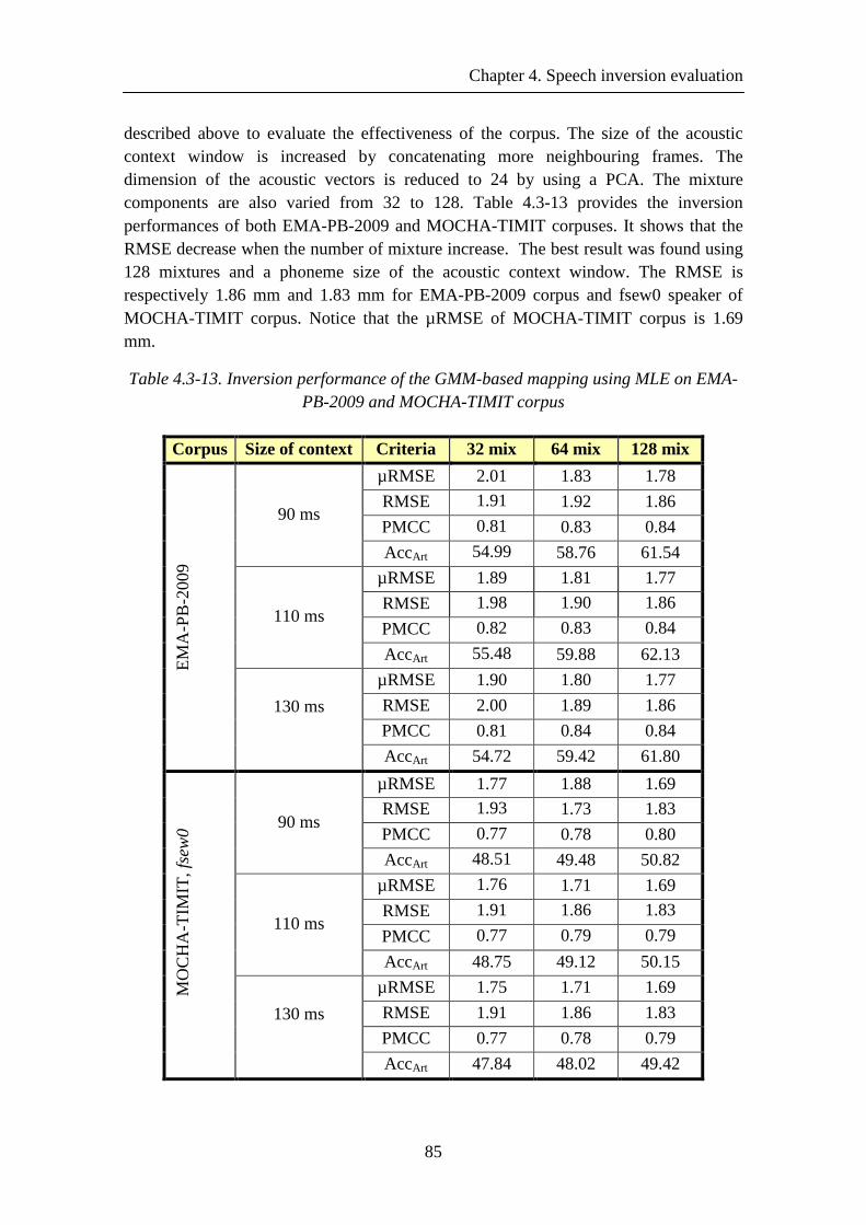
Chapter 4. Speech inversion evaluation
85
described above to evaluate the effectiveness of the corpus. The size of the acoustic context window is increased by concatenating more neighbouring frames. The dimension of the acoustic vectors is reduced to 24 by using a PCA. The mixture components are also varied from 32 to 128. Table 4.3-13 provides the inversion performances of both EMA-PB-2009 and MOCHA-TIMIT corpuses. It shows that the RMSE decrease when the number of mixture increase. The best result was found using 128 mixtures and a phoneme size of the acoustic context window. The RMSE is respectively 1.86 mm and 1.83 mm for EMA-PB-2009 corpus and fsew0 speaker of MOCHA-TIMIT corpus. Notice that the µRMSE of MOCHA-TIMIT corpus is 1.69 mm.
Table 4.3-13. Inversion performance of the GMM-based mapping using MLE on EMA-PB-2009 and MOCHA-TIMIT corpus
Corpus Size of context Criteria 32 mix 64 mix 128 mix
EM
A-P
B-2
009
90 ms
µRMSE 2.01 1.83 1.78
RMSE 1.91 1.92 1.86
PMCC 0.81 0.83 0.84
AccArt 54.99 58.76 61.54
110 ms
µRMSE 1.89 1.81 1.77
RMSE 1.98 1.90 1.86
PMCC 0.82 0.83 0.84
AccArt 55.48 59.88 62.13
130 ms
µRMSE 1.90 1.80 1.77
RMSE 2.00 1.89 1.86
PMCC 0.81 0.84 0.84
AccArt 54.72 59.42 61.80
MO
CH
A-T
IMIT
, fs
ew
0 90 ms
µRMSE 1.77 1.88 1.69
RMSE 1.93 1.73 1.83
PMCC 0.77 0.78 0.80
AccArt 48.51 49.48 50.82
110 ms
µRMSE 1.76 1.71 1.69
RMSE 1.91 1.86 1.83
PMCC 0.77 0.79 0.79
AccArt 48.75 49.12 50.15
130 ms
µRMSE 1.75 1.71 1.69
RMSE 1.91 1.86 1.83
PMCC 0.77 0.78 0.79
AccArt 47.84 48.02 49.42
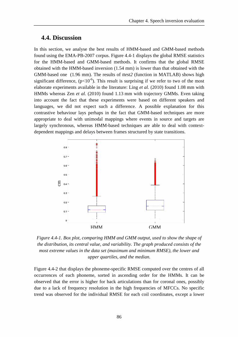
Chapter 4. Speech inversion evaluation
86
4.4. Discussion
In this section, we analyse the best results of HMM-based and GMM-based methods found using the EMA-PB-2007 corpus. Figure 4.4-1 displays the global RMSE statistics for the HMM-based and GMM-based methods. It confirms that the global RMSE obtained with the HMM-based inversion (1.54 mm) is lower than that obtained with the GMM-based one (1.96 mm). The results of ttest2 (function in MATLAB) shows high significant difference, (p<10-6). This result is surprising if we refer to two of the most elaborate experiments available in the literature: Ling et al. (2010) found 1.08 mm with HMMs whereas Zen et al. (2010) found 1.13 mm with trajectory GMMs. Even taking into account the fact that these experiments were based on different speakers and languages, we did not expect such a difference. A possible explanation for this contrastive behaviour lays perhaps in the fact that GMM-based techniques are more appropriate to deal with unimodal mappings where events in source and targets are largely synchronous, whereas HMM-based techniques are able to deal with context-dependent mappings and delays between frames structured by state transitions.
Figure 4.4-1. Box plot, comparing HMM and GMM output, used to show the shape of the distribution, its central value, and variability. The graph produced consists of the most extreme values in the data set (maximum and minimum RMSE), the lower and
upper quartiles, and the median.
Figure 4.4-2 that displays the phoneme-specific RMSE computed over the centres of all occurrences of each phoneme, sorted in ascending order for the HMMs. It can be observed that the error is higher for back articulations than for coronal ones, possibly due to a lack of frequency resolution in the high frequencies of MFCCs. No specific trend was observed for the individual RMSE for each coil coordinates, except a lower
cm
HMM GMM
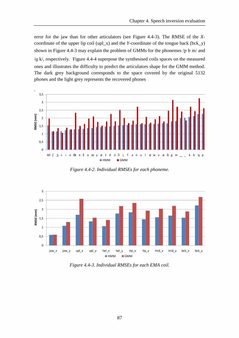
Chapter 4. Speech inversion evaluation
87
error for the jaw than for other articulators (see Figure 4.4-3). The RMSE of the X-coordinate of the upper lip coil (upl_x) and the Y-coordinate of the tongue back (bck_y)
shown in Figure 4.4-3 may explain the problem of GMMs for the phonemes /p b m/ and
/ɡ k/, respectively. Figure 4.4-4 superpose the synthesised coils spaces on the measured
ones and illustrates the difficulty to predict the articulators shape for the GMM method. The dark grey background corresponds to the space covered by the original 5132 phones and the light grey represents the recovered phones
.
0
0,5
1
1,5
2
2,5
3
3,5
All ʃ ʒ s i e œ̃ ɛ ɛ ̃ o œ y ə t d ɔ ɔ̃ j f a n u l ʁ w v ø ɑ̃ g m __ _ k b ɥ p
RM
SE
(m
m)
HMM GMM
Figure 4.4-2. Individual RMSEs for each phoneme.
0
0,5
1
1,5
2
2,5
3
jaw_x jaw_y upl_x upl_y lwl_x lwl_y tip_x tip_y mid_x mid_y bck_x bck_y
RM
SE
(m
m)
HMM GMM
Figure 4.4-3. Individual RMSEs for each EMA coil.
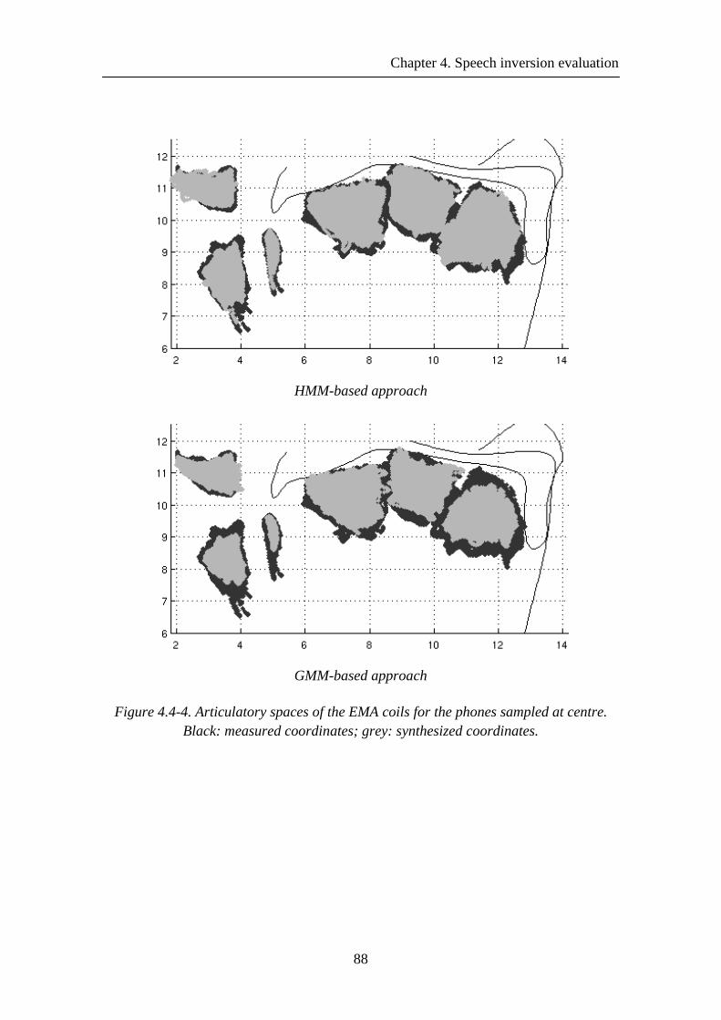
Chapter 4. Speech inversion evaluation
88
HMM-based approach
GMM-based approach
Figure 4.4-4. Articulatory spaces of the EMA coils for the phones sampled at centre. Black: measured coordinates; grey: synthesized coordinates.
Chapter 4. Speech inversion evaluation
89
4.5. Conclusion
This first part of the chapter has presented the evaluation of the two acoustic-to-articulatory speech inversion systems that we have developed. The first system is based on an HMM approach that couples an articulatory speech synthesis system with an acoustic speech recogniser instead of using a direct mapping function. We have made use of various techniques to improve the estimation of the articulatory movements. Concerning the acoustic recognition stage, we have increased the recognition rates by using multi-Gaussians mixtures, context-dependent models, tied states, missing HMMs inheritance. Concerning the articulatory synthesis stage, we have adapted the Maximum Generation Error (MGE) criterium, proposed by Wu et al. (2006; 2008) for speech synthesis, to include an extra training step for the articulatory HMMs in order to improve the estimation of the articulatory trajectories. Context-dependant articulatory HMMs have also brought a significant improvement.
The second system is based on the GMM approach that provides a direct mapping from the acoustic to the articulatory domain. We have shown that articulatory trajectories are improved by using an MMSE-mapping based on a large input context window (about 110 ms) to get more contextual information on input. Articulatory trajectories have been also improved by increasing the number of mixtures. Although the performance of the system was improved, the estimated trajectories still tend to centralisation effects due to the impoverished phonetic contrasts of the GMM-based method.
The performance of our direct signal-to-signal mapping GMM- based approach is currently lower than that of our HMM-based approach. This could be confirmed by a perceptive test, but objective performances are still too different to motivate such an additional benchmark. As mentioned above, this lower score could be explained by two reasons.
First, phonetic information is used explicitly in HMM-based system whereas the GMM-based system only processes contextual frames.
Second, the training of the HMMs is most effective when the training criterion and the task error measurement match. Therefore the HMMs trained to minimise the final reconstruction error are superior to the HMMs trained to maximise the likelihood. On the other hand, the GMMs were trained using the EM algorithm, but the mapping was based on the MMSE-based method. The MLE-based method further improves the inversion mapping performance of the GMMs. The MGE training criterion will be helpful on the re-estimation of the mixture parameters for the HMMs.
The diagonal covariance matrix currently used for each state of the models in the HMM-based system does not take into account the covariance between acoustic and articulatory parameters, whereas the GMM-based system does, by using a full covariance matrix. In the future, we could test if modelling the covariance between
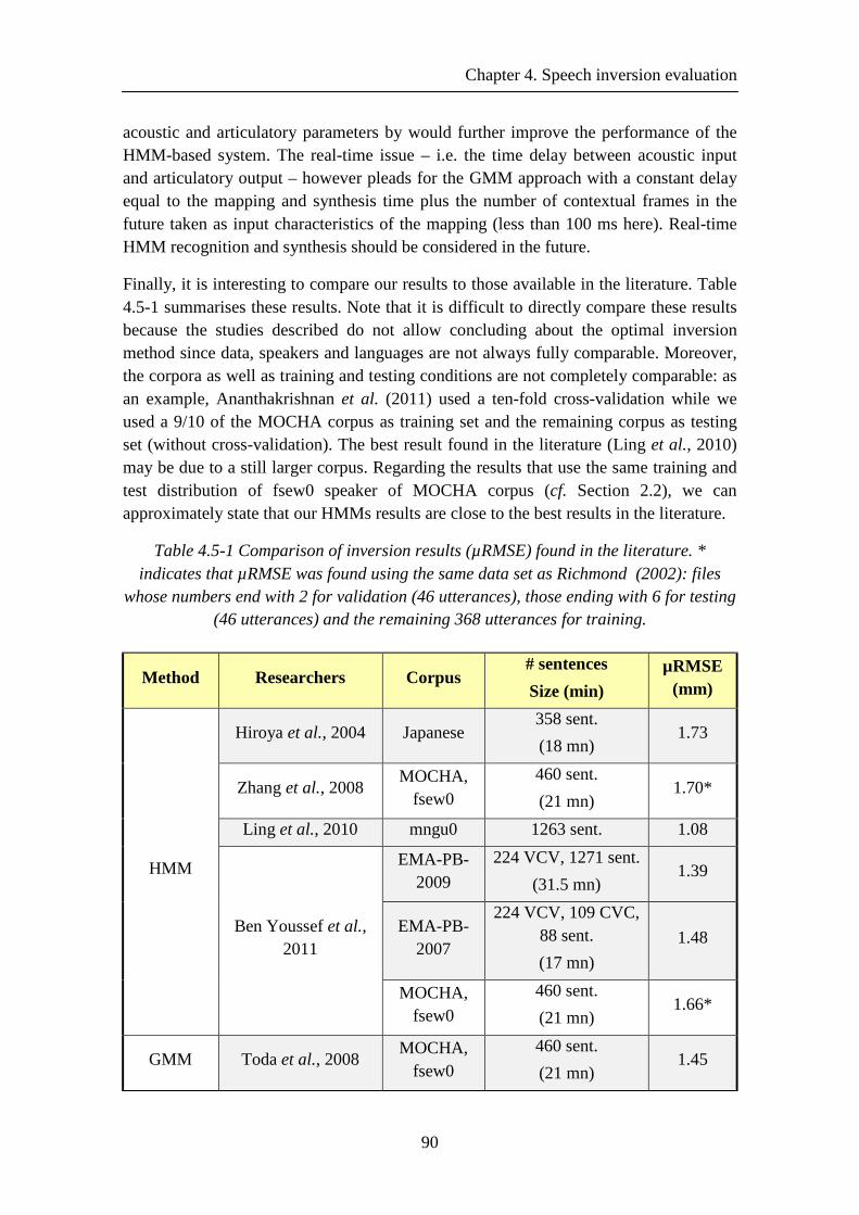
Chapter 4. Speech inversion evaluation
90
acoustic and articulatory parameters by would further improve the performance of the HMM-based system. The real-time issue – i.e. the time delay between acoustic input and articulatory output – however pleads for the GMM approach with a constant delay equal to the mapping and synthesis time plus the number of contextual frames in the future taken as input characteristics of the mapping (less than 100 ms here). Real-time HMM recognition and synthesis should be considered in the future.
Finally, it is interesting to compare our results to those available in the literature. Table 4.5-1 summarises these results. Note that it is difficult to directly compare these results because the studies described do not allow concluding about the optimal inversion method since data, speakers and languages are not always fully comparable. Moreover, the corpora as well as training and testing conditions are not completely comparable: as an example, Ananthakrishnan et al. (2011) used a ten-fold cross-validation while we used a 9/10 of the MOCHA corpus as training set and the remaining corpus as testing set (without cross-validation). The best result found in the literature (Ling et al., 2010) may be due to a still larger corpus. Regarding the results that use the same training and test distribution of fsew0 speaker of MOCHA corpus (cf. Section 2.2), we can approximately state that our HMMs results are close to the best results in the literature.
Table 4.5-1 Comparison of inversion results (µRMSE) found in the literature. * indicates that µRMSE was found using the same data set as Richmond (2002): files
whose numbers end with 2 for validation (46 utterances), those ending with 6 for testing (46 utterances) and the remaining 368 utterances for training.
Method Researchers Corpus # sentences
Size (min)
µRMSE (mm)
HMM
Hiroya et al., 2004 Japanese 358 sent.
(18 mn) 1.73
Zhang et al., 2008 MOCHA,
fsew0
460 sent.
(21 mn) 1.70*
Ling et al., 2010 mngu0 1263 sent. 1.08
Ben Youssef et al., 2011
EMA-PB-2009
224 VCV, 1271 sent.
(31.5 mn) 1.39
EMA-PB-2007
224 VCV, 109 CVC, 88 sent.
(17 mn)
1.48
MOCHA, fsew0
460 sent.
(21 mn) 1.66*
GMM Toda et al., 2008 MOCHA,
fsew0
460 sent.
(21 mn) 1.45
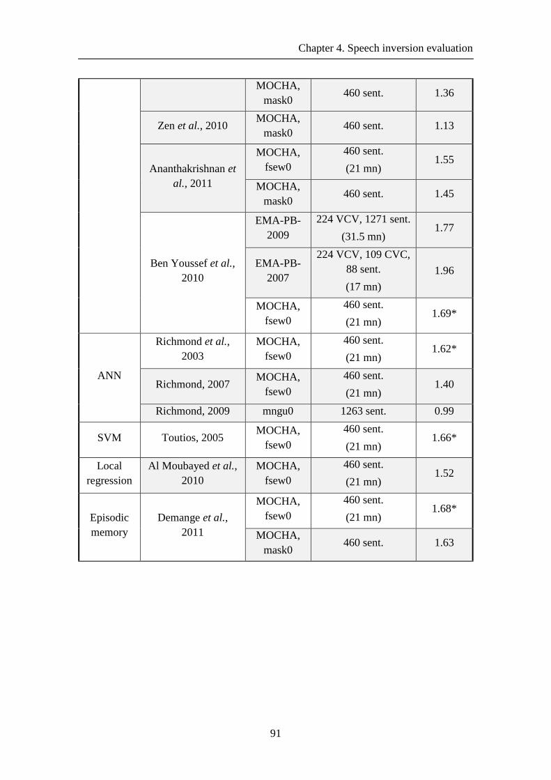
Chapter 4. Speech inversion evaluation
91
MOCHA, mask0
460 sent. 1.36
Zen et al., 2010 MOCHA,
mask0 460 sent. 1.13
Ananthakrishnan et al., 2011
MOCHA, fsew0
460 sent.
(21 mn) 1.55
MOCHA, mask0
460 sent. 1.45
Ben Youssef et al., 2010
EMA-PB-2009
224 VCV, 1271 sent.
(31.5 mn) 1.77
EMA-PB-2007
224 VCV, 109 CVC, 88 sent.
(17 mn)
1.96
MOCHA, fsew0
460 sent.
(21 mn) 1.69*
ANN
Richmond et al., 2003
MOCHA, fsew0
460 sent.
(21 mn) 1.62*
Richmond, 2007 MOCHA,
fsew0
460 sent.
(21 mn) 1.40
Richmond, 2009 mngu0 1263 sent. 0.99
SVM Toutios, 2005 MOCHA,
fsew0
460 sent.
(21 mn) 1.66*
Local regression
Al Moubayed et al., 2010
MOCHA, fsew0
460 sent.
(21 mn) 1.52
Episodic memory
Demange et al., 2011
MOCHA, fsew0
460 sent.
(21 mn) 1.68*
MOCHA, mask0
460 sent. 1.63

Chapter 5. Toward a multi-speaker visual articulatory feedback system
93
Chapter 5. Toward a multi-speaker visual articulatory feedback system
5.1. Introduction
Visual articulatory feedback systems aim at providing a speaker with visual information about his/her own articulation.
Ideally, our aim would be to provide any speaker in any L1 or L2 language with his / her own articulators animation. This is obviously a challenge impossible to manage at present. Previous chapters have described the acoustic-to-articulatory inversion that we have developed for the reference speaker used to build the GIPSA-lab talking head. We will describe in the present chapter the visual articulatory feedback system that we have developed for this speaker in his L1 language.
Since our goal is to provide “any” speaker with visual articulatory feedback, the inversion system needs to be robust and easy to adapt. We have developed an acoustic adaptation stage that allows various speakers to use the system, though the visual articulatory feedback is restricted to the talking head of the reference subject, and does not feature the articulatory characteristics specific to the speaker. Figure 5.1-1 shows the three components of our visual articulatory feedback system: (1) the speech inversion mapping based on statistical models trained using acoustic and EMA corpus recorded by a French speaker presented in chapter 2, (2) the acoustic speaker adaptation stage that will describes in the present chapter and (3) the animation of the talking head from inversed EMA trajectories.
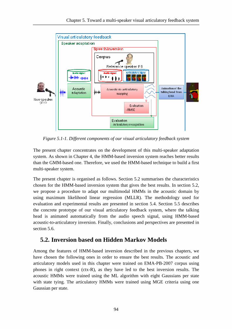
Chapter 5. Toward a multi-speaker visual articulatory feedback system
94
Figure 5.1-1. Different components of our visual articulatory feedback system
The present chapter concentrates on the development of this multi-speaker adaptation system. As shown in Chapter 4, the HMM-based inversion system reaches better results than the GMM-based one. Therefore, we used the HMM-based technique to build a first multi-speaker system.
The present chapter is organised as follows. Section 5.2 summarises the characteristics chosen for the HMM-based inversion system that gives the best results. In section 5.2, we propose a procedure to adapt our multimodal HMMs in the acoustic domain by using maximum likelihood linear regression (MLLR). The methodology used for evaluation and experimental results are presented in section 5.4. Section 5.5 describes the concrete prototype of our visual articulatory feedback system, where the talking head is animated automatically from the audio speech signal, using HMM-based acoustic-to-articulatory inversion. Finally, conclusions and perspectives are presented in section 5.6.
5.2. Inversion based on Hidden Markov Models
Among the features of HMM-based inversion described in the previous chapters, we have chosen the following ones in order to ensure the best results. The acoustic and articulatory models used in this chapter were trained on EMA-PB-2007 corpus using phones in right context (ctx-R), as they have led to the best inversion results. The acoustic HMMs were trained using the ML algorithm with eight Gaussians per state with state tying. The articulatory HMMs were trained using MGE criteria using one Gaussian per state.
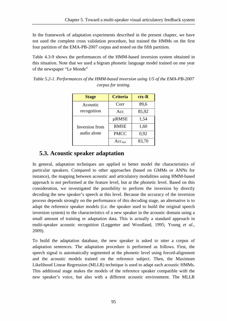
Chapter 5. Toward a multi-speaker visual articulatory feedback system
95
In the framework of adaptation experiments described in the present chapter, we have not used the complete cross validation procedure, but trained the HMMs on the first four partition of the EMA-PB-2007 corpus and tested on the fifth partition.
Table 4.3-9 shows the performances of the HMM-based inversion system obtained in this situation. Note that we used a bigram phonetic language model trained on one year of the newspaper “Le Monde”
Table 5.2-1. Performances of the HMM-based inversion using 1/5 of the EMA-PB-2007 corpus for testing.
Stage Criteria ctx-R
Acoustic recognition
Corr 89,6
Acc 85,92
Inversion from audio alone
µRMSE 1,54
RMSE 1,60
PMCC 0,92
AccArt 83,70
5.3. Acoustic speaker adaptation
In general, adaptation techniques are applied to better model the characteristics of particular speakers. Compared to other approaches (based on GMMs or ANNs for instance), the mapping between acoustic and articulatory modalities using HMM-based approach is not performed at the feature level, but at the phonetic level. Based on this consideration, we investigated the possibility to perform the inversion by directly decoding the new speaker’s speech at this level. Because the accuracy of the inversion process depends strongly on the performance of this decoding stage, an alternative is to adapt the reference speaker models (i.e. the speaker used to build the original speech inversion system) to the characteristics of a new speaker in the acoustic domain using a small amount of training or adaptation data. This is actually a standard approach in multi-speaker acoustic recognition (Leggetter and Woodland, 1995; Young et al., 2009).
To build the adaptation database, the new speaker is asked to utter a corpus of adaptation sentences. The adaptation procedure is performed as follows. First, the speech signal is automatically segmented at the phonetic level using forced-alignment and the acoustic models trained on the reference subject. Then, the Maximum Likelihood Linear Regression (MLLR) technique is used to adapt each acoustic HMMs. This additional stage makes the models of the reference speaker compatible with the new speaker’s voice, but also with a different acoustic environment. The MLLR
Chapter 5. Toward a multi-speaker visual articulatory feedback system
96
approach estimates linear transformations for models parameters to maximise the likelihood of the adaptation data (Leggetter and Woodland, 1995).
MLLR-Mean updates the model mean parameters to maximise the likelihood of the adaptation data uttered by a new speaker. The other HMM parameters are not adapted since the main differences between speakers are assumed to be characterised by the means. In other words, the adapted means µ̂ are defined as
ˆ .b Aµ µ= + (5.3-1)
where µ represents the n-dimensional vector of means, A the n n× transformation matrix, and b represents a bias vector. This notation can also be written as in equation
(5.3-2), where [ ]1;ξ µ= and [ ],W b A=
ˆ .Wµ ξ= (5.3-2)
The transformation matrix W, defined for each model, is estimated such that the likelihood of the adaptation data is maximised and satisfies
( )argmax p WW
W P O λ= (5.3-3)
where Op are the p observed utterances associated with the model, and Wλ is the
adapted model.
To improve the flexibility of the adaptation process, the matrix W in equation (5.3-3) should not be estimated for every mixture component separately. Instead, it is possible to combine several mixtures in one regression class depending on the amount of existing adaptation data. A global transform class is applied to every Gaussian component in the model set when a small amount of data is available. When more adaptation data become available, the number of transformations can be increased and improves the adaptation stage. For instance every vector of means in one class is transformed by the same matrix. This has the advantage of clustering the related mixture components that should be transformed in a similar way (e.g. mixture components that are acoustically or phonetically related), and of increasing the amount of adaptation data for one matrix.
Depending on the available amount of adaptation data, MLLR use a regression class tree to group the Gaussians in a set of model and to choose the set of transformations to be estimated. The tying of transformation classes makes possible to adapt Gaussians that do not have any observations at all. Consequently, all models can be adapted and the adaptation process is dynamically refined when more adaptation data becomes available.
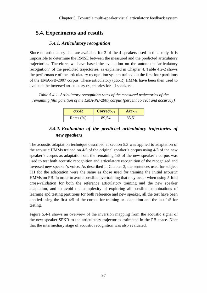
Chapter 5. Toward a multi-speaker visual articulatory feedback system
97
5.4. Experiments and results
5.4.1. Articulatory recognition
Since no articulatory data are available for 3 of the 4 speakers used in this study, it is impossible to determine the RMSE between the measured and the predicted articulatory trajectories. Therefore, we have based the evaluation on the automatic “articulatory recognition” of the predicted trajectories, as explained in Chapter 4. Table 4.2-2 shows the performance of the articulatory recognition system trained on the first four partitions of the EMA-PB-2007 corpus. These articulatory (ctx-R) HMMs have been then used to evaluate the inversed articulatory trajectories for all speakers.
Table 5.4-1. Articulatory recognition rates of the measured trajectories of the remaining fifth partition of the EMA-PB-2007 corpus (percent correct and accuracy)
ctx-R CorrectArt AccArt
Rates (%) 89,54 85,51
5.4.2. Evaluation of the predicted articulatory trajectories of new speakers
The acoustic adaptation technique described at section 5.3 was applied to adaptation of the acoustic HMMs trained on 4/5 of the original speaker’s corpus using 4/5 of the new speaker’s corpus as adaptation set; the remaining 1/5 of the new speaker’s corpus was used to test both acoustic recognition and articulatory recognition of the recognised and inversed new speaker’s voice. As described in Chapter 3, the sentences used for subject TH for the adaptation were the same as those used for training the initial acoustic HMMs on PB. In order to avoid possible overtraining that may occur when using 5-fold cross-validation for both the reference articulatory training and the new speaker adaptation, and to avoid the complexity of exploring all possible combinations of learning and testing partitions for both reference and new speaker, all the test have been applied using the first 4/5 of the corpus for training or adaptation and the last 1/5 for testing.
Figure 5.4-1 shows an overview of the inversion mapping from the acoustic signal of the new speaker SPKR to the articulatory trajectories estimated in the PB space. Note that the intermediary stage of acoustic recognition was also evaluated.
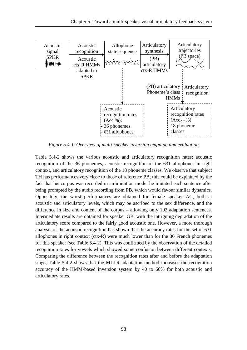
Chapter 5. Toward a multi-speaker visual articulatory feedback system
98
Figure 5.4-1. Overview of multi-speaker inversion mapping and evaluation
Table 5.4-2 shows the various acoustic and articulatory recognition rates: acoustic recognition of the 36 phonemes, acoustic recognition of the 631 allophones in right context, and articulatory recognition of the 18 phoneme classes. We observe that subject TH has performances very close to those of reference PB; this could be explained by the fact that his corpus was recorded in an imitation mode: he imitated each sentence after being prompted by the audio recording from PB, which would favour similar dynamics. Oppositely, the worst performances are obtained for female speaker AC, both at acoustic and articulatory levels, which may be ascribed to the sex difference, and the difference in size and content of the corpus – allowing only 192 adaptation sentences. Intermediate results are obtained for speaker GB, with the intriguing degradation of the articulatory score compared to the fairly good acoustic one. However, a more thorough analysis of the acoustic recognition has shown that the accuracy rates for the set of 631 allophones in right context (ctx-R) were much lower than for the 36 French phonemes for this speaker (see Table 5.4-2). This was confirmed by the observation of the detailed recognition rates for vowels which showed some confusion between different contexts. Comparing the difference between the recognition rates after and before the adaptation stage, Table 5.4-2 shows that the MLLR adaptation method increases the recognition accuracy of the HMM-based inversion system by 40 to 60% for both acoustic and articulatory rates.
Articulatory trajectories (PB space)
Allophone state sequence
Acoustic signal SPKR
Acoustic recognition
Acoustic ctx-R HMMs
adapted to SPKR
Articulatory synthesis
(PB) articulatory
ctx-R HMMs
Articulatory recognition rates (AccArt %):
- 18 phoneme classes
Acoustic recognition rates (Acc %):
- 36 phonemes - 631 allophones
(PB) articulatory Phoneme’s class
HMMs
Articulatory recognition
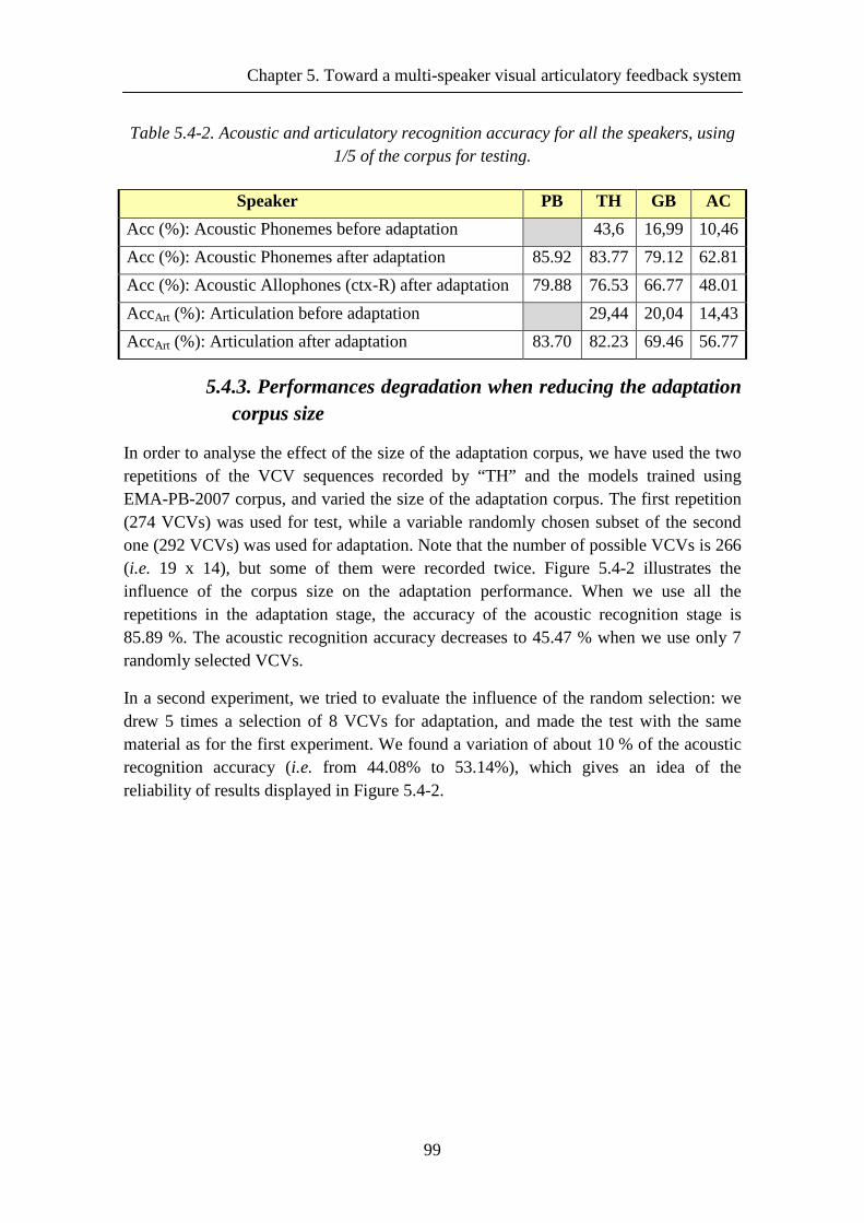
Chapter 5. Toward a multi-speaker visual articulatory feedback system
99
Table 5.4-2. Acoustic and articulatory recognition accuracy for all the speakers, using 1/5 of the corpus for testing.
Speaker PB TH GB AC
Acc (%): Acoustic Phonemes before adaptation 43,6 16,99 10,46
Acc (%): Acoustic Phonemes after adaptation 85.92 83.77 79.12 62.81
Acc (%): Acoustic Allophones (ctx-R) after adaptation 79.88 76.53 66.77 48.01
AccArt (%): Articulation before adaptation 29,44 20,04 14,43
AccArt (%): Articulation after adaptation 83.70 82.23 69.46 56.77
5.4.3. Performances degradation when reducing the adaptation corpus size
In order to analyse the effect of the size of the adaptation corpus, we have used the two repetitions of the VCV sequences recorded by “TH” and the models trained using EMA-PB-2007 corpus, and varied the size of the adaptation corpus. The first repetition (274 VCVs) was used for test, while a variable randomly chosen subset of the second one (292 VCVs) was used for adaptation. Note that the number of possible VCVs is 266 (i.e. 19 x 14), but some of them were recorded twice. Figure 5.4-2 illustrates the influence of the corpus size on the adaptation performance. When we use all the repetitions in the adaptation stage, the accuracy of the acoustic recognition stage is 85.89 %. The acoustic recognition accuracy decreases to 45.47 % when we use only 7 randomly selected VCVs.
In a second experiment, we tried to evaluate the influence of the random selection: we drew 5 times a selection of 8 VCVs for adaptation, and made the test with the same material as for the first experiment. We found a variation of about 10 % of the acoustic recognition accuracy (i.e. from 44.08% to 53.14%), which gives an idea of the reliability of results displayed in Figure 5.4-2.
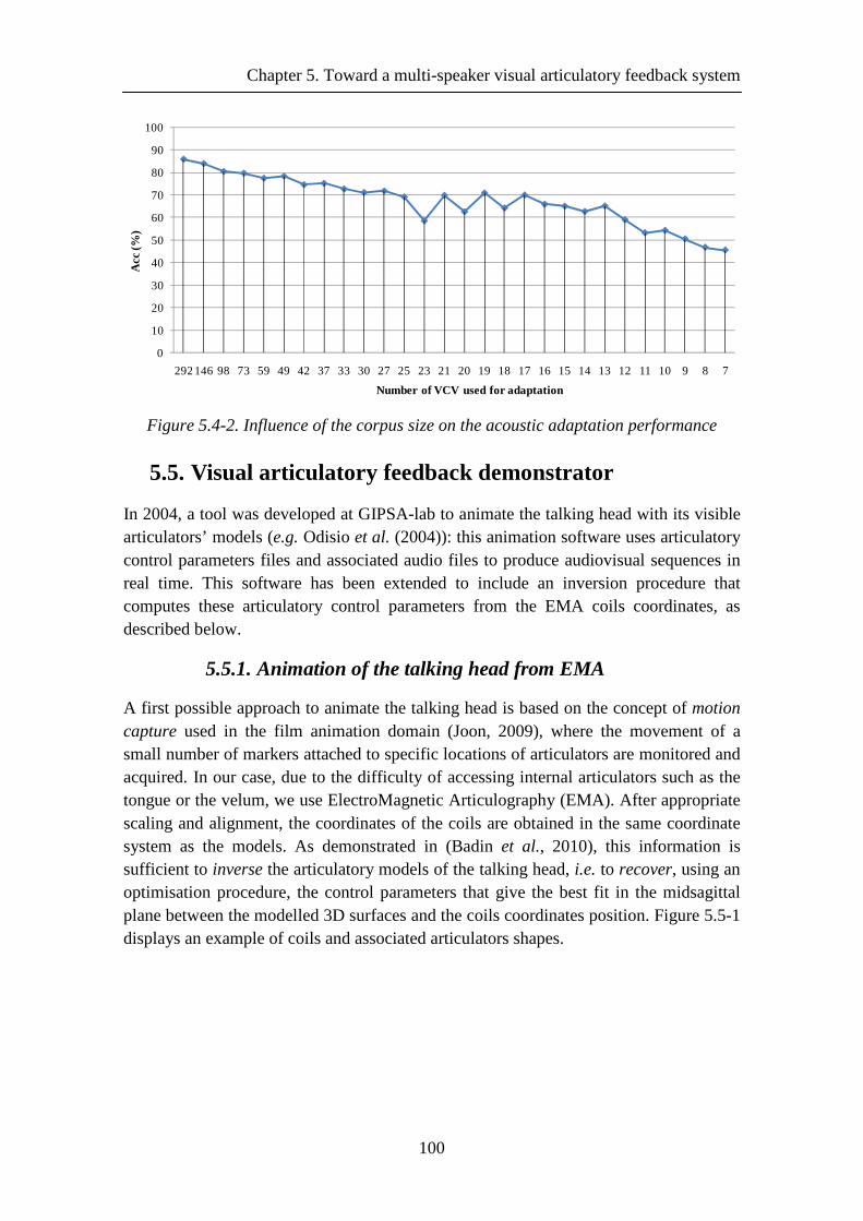
Chapter 5. Toward a multi-speaker visual articulatory feedback system
100
0
10
20
30
40
50
60
70
80
90
100
292146 98 73 59 49 42 37 33 30 27 25 23 21 20 19 18 17 16 15 14 13 12 11 10 9 8 7
Acc
(%)
Number of VCV used for adaptation
Figure 5.4-2. Influence of the corpus size on the acoustic adaptation performance
5.5. Visual articulatory feedback demonstrator
In 2004, a tool was developed at GIPSA-lab to animate the talking head with its visible articulators’ models (e.g. Odisio et al. (2004)): this animation software uses articulatory control parameters files and associated audio files to produce audiovisual sequences in real time. This software has been extended to include an inversion procedure that computes these articulatory control parameters from the EMA coils coordinates, as described below.
5.5.1. Animation of the talking head from EMA
A first possible approach to animate the talking head is based on the concept of motion capture used in the film animation domain (Joon, 2009), where the movement of a small number of markers attached to specific locations of articulators are monitored and acquired. In our case, due to the difficulty of accessing internal articulators such as the tongue or the velum, we use ElectroMagnetic Articulography (EMA). After appropriate scaling and alignment, the coordinates of the coils are obtained in the same coordinate system as the models. As demonstrated in (Badin et al., 2010), this information is sufficient to inverse the articulatory models of the talking head, i.e. to recover, using an optimisation procedure, the control parameters that give the best fit in the midsagittal plane between the modelled 3D surfaces and the coils coordinates position. Figure 5.5-1 displays an example of coils and associated articulators shapes.
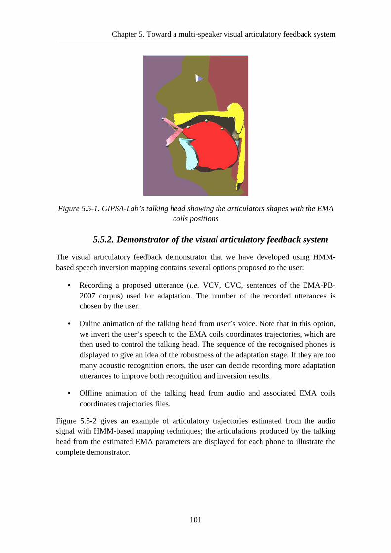
Chapter 5. Toward a multi-speaker visual articulatory feedback system
101
Figure 5.5-1. GIPSA-Lab’s talking head showing the articulators shapes with the EMA coils positions
5.5.2. Demonstrator of the visual articulatory feedback system
The visual articulatory feedback demonstrator that we have developed using HMM-based speech inversion mapping contains several options proposed to the user:
• Recording a proposed utterance (i.e. VCV, CVC, sentences of the EMA-PB-2007 corpus) used for adaptation. The number of the recorded utterances is chosen by the user.
• Online animation of the talking head from user’s voice. Note that in this option, we invert the user’s speech to the EMA coils coordinates trajectories, which are then used to control the talking head. The sequence of the recognised phones is displayed to give an idea of the robustness of the adaptation stage. If they are too many acoustic recognition errors, the user can decide recording more adaptation utterances to improve both recognition and inversion results.
• Offline animation of the talking head from audio and associated EMA coils coordinates trajectories files.
Figure 5.5-2 gives an example of articulatory trajectories estimated from the audio signal with HMM-based mapping techniques; the articulations produced by the talking head from the estimated EMA parameters are displayed for each phone to illustrate the complete demonstrator.
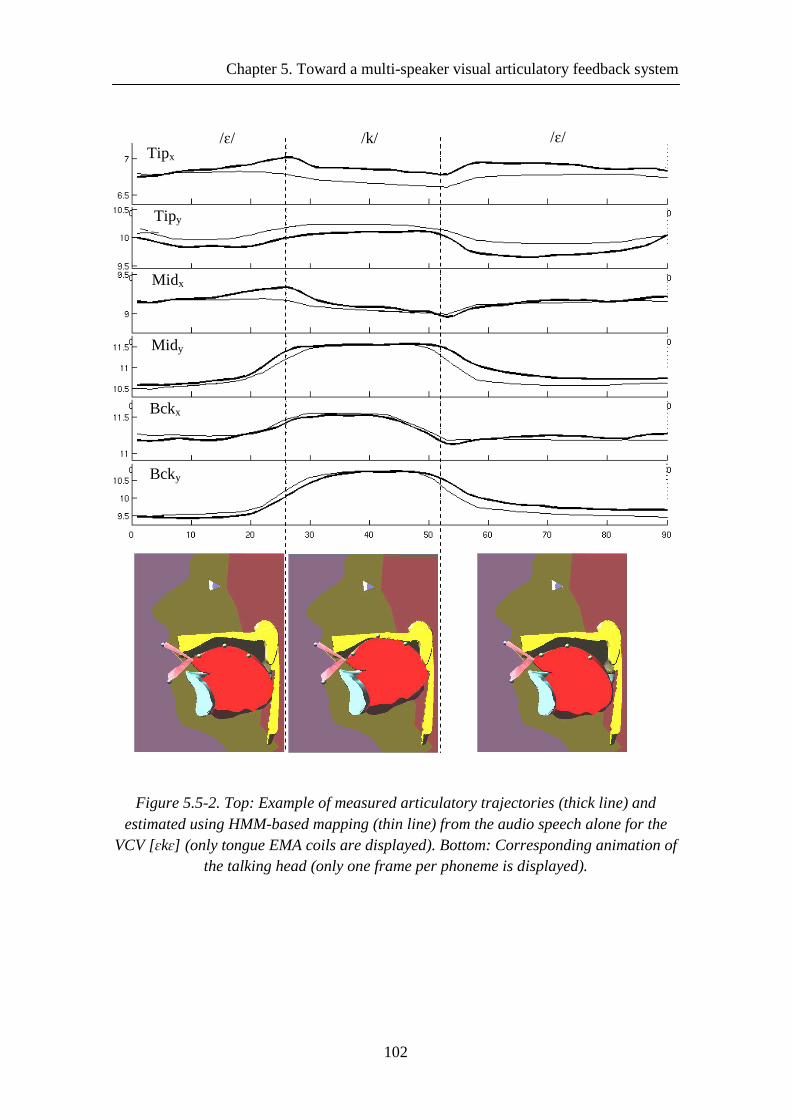
Chapter 5. Toward a multi-speaker visual articulatory feedback system
102
Figure 5.5-2. Top: Example of measured articulatory trajectories (thick line) and estimated using HMM-based mapping (thin line) from the audio speech alone for the
VCV [ɛkɛ] (only tongue EMA coils are displayed). Bottom: Corresponding animation of the talking head (only one frame per phoneme is displayed).
Tipx
Bcky
Bckx
Midy
Midx
Tipy
/ɛ/ /ɛ/ /k/
Chapter 5. Toward a multi-speaker visual articulatory feedback system
103
5.6. Conclusion
This chapter has described a multi-speaker HMM-based acoustic-to-articulatory speech inversion system that has allowed us to develop a visual articulatory feedback demonstrator.
As a first step toward a multi-speaker system, we investigated the use of an MLLR model adaptation technique. The quality of the articulatory trajectories was evaluated by measuring the performance of an articulatory HMM-based phonetic decoder. Recognition accuracies range between 56.8 % and 82.2 % for three speakers, compared to 83.7 % for the original speaker, demonstrating the interest of the method.
It is now needed to test more speakers, and to study more explicitly the influence of the nature and size of the adaptation corpus.

Chapter 6. Face-to-tongue mapping
105
Chapter 6. Face-to-tongue mapping
6.1. Introduction
The techniques described in Chapter 2 for acoustic-to-articulatory mapping can be applied in a straightforward manner to face-to-tongue mapping, i.e. reconstructing tongue shape from face shape. Since more than a decade, the question whether tongue shape can be predicted from lips and face shape is indeed still debated ((Yehia et al., 1998), (Jiang et al., 2002), (Bailly and Badin, 2002), (Engwall and Beskow, 2003), (Beskow et al., 2003)). So far, these studies were all based on linear modelling. The present Chapter revisits this problem with the more sophisticated mapping techniques that we have described above, and compares the results with those obtained with linear models using the articulatory data of the EMA-PB-2007 corpus.
The present chapter is organised as follows. Section 6.2 presents the state-of-the-art in Face-to-Tongue inversion, Section 6.3 describe the three approaches explored and the evaluation of the results. Section 6.4 presents the discussion. Finally, conclusions are presented in section 6.5.
6.2. State-of-the-art
All the studies found in the literature used similar articulatory data: one point on the jaw and three points on the tongue recorded by ElectroMagnetoGraphy (EMA), simultaneously with face and lip movements captured by a marker tracking devices (12 or 18 Optotrak points in Yehia et al. (1998), 17 Qualisys points in Jiang et al. (2002), 25 Qualisys points in Engwall and Beskow (2003) and Beskow et al. (2003)). By exception, Bailly and Badin (2002) use midsagittal contours traced from X-ray pictures: the tongue is represented by the parameters of a midsagittal articulatory model that fits its shape, while the face and lips are represented by those of another associated 2D model. A tongue model is also used in Engwall and Beskow (2003). Note that tongue and face / lips data in Yehia et al. (1998) were not acquired simultaneously and had to be time aligned by Dynamic Time Warping (DTW).
The size and nature of the corpus vary a lot: a few sentences repeated 5 times by one American English speaker (total ~400 syllables) and 4 times by one Japanese speaker (total ~400 syllables) in Yehia et al. (1998); 69 CV syllables with /a, i, u/ and 23 consonants, and 3 sentences repeated 4 times (total ~520 syllables) by four American English speakers in Jiang et al. (2002); 45 frames selected at the centre of VCV syllables produced by one French speaker in Bailly and Badin (2002); 63 VCV with /a i u/ context uttered once by one Swedish speaker in Engwall and Beskow (2003); 138
Chapter 6. Face-to-tongue mapping
106
symmetric VC1{C2C3}VCV, 41 CVC and 270 short sentences (total ~2500 syllables) uttered by one Swedish speaker in Beskow et al. (2003).
All studies use Multi Linear Regression (MLR) to predict tongue data from face data. The inversion is assessed by computing the Pearson product-moment correlation coefficient (PMCC) between measured and predicted data. In a jack-knife training procedure, the data are split into n parts of which (n -1) are used to determine the MLR coefficients, and to predict the n-th remaining part. The PMCC coefficient is the average over the n values of the correlation coefficients between obtained by the jack-knife procedure. The factor n is set to 4 or 5 in Yehia et al. (1998) and Jiang et al. (2002), to 1 in Bailly and Badin (2002), and to 10 in Engwall and Beskow (2003) and Beskow et al. (2003).
Results are summarised in Table 6.2-1. The first line refers to tongue coils receptors: (Tx, Ty), (Mx, My) and (Bx, By) correspond to the horizontal and vertical midsagittal coordinates of the coils attached respectively to the tongue tip, the tongue middle, and the tongue back; moreover, G refers to the PMCC computed over the six coordinates. For (Bailly and Badin, 2002) and (Engwall and Beskow, 2003), TB, TD, TT and TA (light gray in Table 6.2-1) refer respectively to the tongue Body, Dorsum, Tip and Advance control parameters of the articulatory tongue model. From their results, (Yehia et al., 1998) claim that the tongue can be recovered reasonably well from facial motion; however, if we exclude jaw and lips coils from their predicted data, we find only medium correlations (0.65 – 0.79). Medium to high correlations are found in (Jiang et al., 2002), whereas lower correlations are obtained by (Engwall and Beskow, 2003), and also by (Bailly and Badin, 2002) and (Engwall and Beskow, 2003) when using an articulatory model to track speech movements. On a larger corpus, (Beskow et al., 2003) gets a still lower global correlation.
Interestingly, tongue tip (either Ty or TT) appears to be the tongue region best recovered in all studies: (Bailly and Badin, 2002) suggests that this may be ascribed to the fact that the jaw is an articulator with a strong influence on both labial and lingual shapes.
Phonetic context has a clear influence on the results: Jiang et al. (2002) and (Bailly and Badin (2002) note that results are better for C/a/ syllables than for C/i/ and C/u/ syllables, while Engwall and Beskow (2003) describes a more complex pattern. Bailly and Badin (2002) remark that articulations associating a jaw/tongue/lips synergy along the axis closed/front (e.g. [i]) vs. open/back (e.g. [a]) are more accurately recovered than those requiring constrictions deviating from this synergy. In complement, Engwall and Beskow (2003) note that face information is insufficient to accurately predict a non alveolar vocal tract constriction, which is in line with Bailly and Badin (2002).
The fact that the lowest mean correlation is obtained in the study with the largest corpus (Beskow et al., 2003), in complement to the fact that correlations are higher for CVs in context than for sentences (Jiang et al., 2002) suggests that linear methods may be
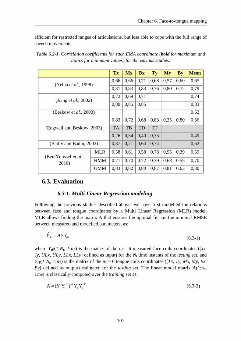
Chapter 6. Face-to-tongue mapping
107
efficient for restricted ranges of articulations, but less able to cope with the full range of speech movements.
Table 6.2-1. Correlation coefficients for each EMA coordinate (bold for maximum and italics for minimum values) for the various studies.
Tx Mx Bx Ty My By Mean
(Yehia et al., 1998) 0,66 0,66 0,71 0,68 0,57 0,60 0,65
0,81 0,83 0,83 0,76 0,80 0,72 0,79
(Jiang et al., 2002) 0,72 0,69 0,71 0,74
0,80 0,85 0,85 0,83
(Beskow et al., 2003) 0,52
(Engwall and Beskow, 2003)
0,83 0,72 0,68 0,83 0,35 0,80 0,66
TA TB TD TT
0,26 0,54 0,40 0,75 0,49
(Bailly and Badin, 2002) 0,37 0,71 0,64 0,74 0,62
(Ben Youssef et al., 2010)
MLR 0,58 0,61 0,58 0,78 0,55 0,39 0,59
HMM 0.71 0.70 0.72 0.79 0.68 0.55 0,70
GMM 0,83 0,82 0,80 0,87 0,81 0,63 0,80
6.3. Evaluation
6.3.1. Multi Linear Regression modeling
Following the previous studies described above, we have first modelled the relations between face and tongue coordinates by a Multi Linear Regression (MLR) model. MLR allows finding the matrix A that ensures the optimal fit, i.e. the minimal RMSE between measured and modelled parameters, as:
tFtT YAY ×=ˆ
(6.3-1)
where YtF(1:Nt, 1:nF) is the matrix of the nF = 6 measured face coils coordinates ([Jx, Jy, ULx, ULy, LLx, LLy] defined as input) for the Nt time instants of the testing set, and ŶtT(1:Nt, 1:nT) is the matrix of the nT = 6 tongue coils coordinates ([Tx, Ty, Mx, My, Bx, By] defined as output) estimated for the testing set. The linear model matrix A(1:nF, 1:nT) is classically computed over the training set as:
TTTF
1FF YY)Y(Y A −= (6.3-2)
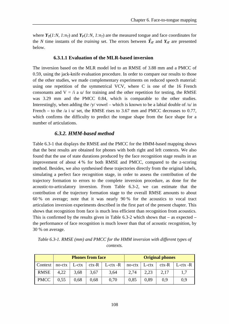
Chapter 6. Face-to-tongue mapping
108
where YT(1:N, 1:nT) and YF(1:N, 1:nT) are the measured tongue and face coordinates for the N time instants of the training set. The errors between ŶtT and YtT are presented below.
6.3.1.1 Evaluation of the MLR-based inversion
The inversion based on the MLR model led to an RMSE of 3.88 mm and a PMCC of 0.59, using the jack-knife evaluation procedure. In order to compare our results to those of the other studies, we made complementary experiments on reduced speech material: using one repetition of the symmetrical VCV, where C is one of the 16 French consonants and V = /i a u/ for training and the other repetition for testing, the RMSE was 3.29 mm and the PMCC 0.84, which is comparable to the other studies. Interestingly, when adding the /y/ vowel – which is known to be a labial double of /u/ in French – to the /a i u/ set, the RMSE rises to 3.67 mm and PMCC decreases to 0.77, which confirms the difficulty to predict the tongue shape from the face shape for a number of articulations.
6.3.2. HMM-based method
Table 6.3-1 that displays the RMSE and the PMCC for the HMM-based mapping shows that the best results are obtained for phones with both right and left contexts. We also found that the use of state durations produced by the face recognition stage results in an improvement of about 4 % for both RMSE and PMCC, compared to the z-scoring method. Besides, we also synthesised these trajectories directly from the original labels, simulating a perfect face recognition stage, in order to assess the contribution of the trajectory formation to errors to the complete inversion procedure, as done for the acoustic-to-articulatory inversion. From Table 6.3-2, we can estimate that the contribution of the trajectory formation stage to the overall RMSE amounts to about 60 % on average; note that it was nearly 90 % for the acoustics to vocal tract articulation inversion experiments described in the first part of the present chapter. This shows that recognition from face is much less efficient than recognition from acoustics. This is confirmed by the results given in Table 6.3-2 which shows that – as expected – the performance of face recognition is much lower than that of acoustic recognition, by 30 % on average.
Table 6.3-1. RMSE (mm) and PMCC for the HMM inversion with different types of contexts.
Phones from face Original phones
Context no-ctx L-ctx ctx-R L-ctx -R no-ctx L-ctx ctx-R L-ctx -R
RMSE 4,22 3,68 3,67 3,64 2,74 2,23 2,17 1,7
PMCC 0,55 0,68 0,68 0,70 0,85 0,89 0,9 0,9
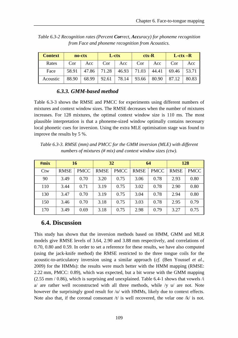
Chapter 6. Face-to-tongue mapping
109
Table 6.3-2 Recognition rates (Percent Correct, Accuracy) for phoneme recognition from Face and phoneme recognition from Acoustics.
Context no-ctx L-ctx ctx-R L-ctx –R
Rates Cor Acc Cor Acc Cor Acc Cor Acc
Face 58.91 47.86 71.28 46.93 71.03 44.41 69.46 53.71
Acoustic 88.90 68.99 92.61 78.14 93.66 80.90 87.12 80.83
6.3.3. GMM-based method
Table 6.3-3 shows the RMSE and PMCC for experiments using different numbers of mixtures and context window sizes. The RMSE decreases when the number of mixtures increases. For 128 mixtures, the optimal context window size is 110 ms. The most plausible interpretation is that a phoneme-sized window optimally contains necessary local phonetic cues for inversion. Using the extra MLE optimisation stage was found to improve the results by 5 %.
Table 6.3-3. RMSE (mm) and PMCC for the GMM inversion (MLE) with different numbers of mixtures (# mix) and context window sizes (ctw).
#mix 16 32 64 128
Ctw RMSE PMCC RMSE PMCC RMSE PMCC RMSE PMCC
90 3.49 0.70 3.20 0.75 3.06 0.78 2.93 0.80
110 3.44 0.71 3.19 0.75 3.02 0.78 2.90 0.80
130 3.47 0.70 3.19 0.75 3.04 0.78 2.94 0.80
150 3.46 0.70 3.18 0.75 3.03 0.78 2.95 0.79
170 3.49 0.69 3.18 0.75 2.98 0.79 3.27 0.75
6.4. Discussion
This study has shown that the inversion methods based on HMM, GMM and MLR models give RMSE levels of 3.64, 2.90 and 3.88 mm respectively, and correlations of 0.70, 0.80 and 0.59. In order to set a reference for these results, we have also computed (using the jack-knife method) the RMSE restricted to the three tongue coils for the acoustic-to-articulatory inversion using a similar approach (cf. (Ben Youssef et al., 2009) for the HMMs): the results were much better with the HMM mapping (RMSE: 2.22 mm, PMCC: 0.89), which was expected, but a bit worse with the GMM mapping (2.55 mm / 0.86), which is surprising and unexplained. Table 6.4-1 shows that vowels /i a/ are rather well reconstructed with all three methods, while /y u/ are not. Note however the surprisingly good result for /u/ with HMMs, likely due to context effects. Note also that, if the coronal consonant /t/ is well recovered, the velar one /k/ is not.
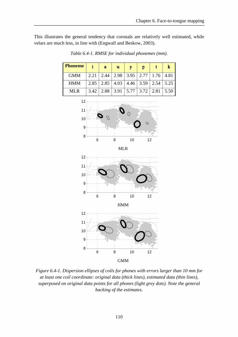
Chapter 6. Face-to-tongue mapping
110
This illustrates the general tendency that coronals are relatively well estimated, while velars are much less, in line with (Engwall and Beskow, 2003).
Table 6.4-1. RMSE for individual phonemes (mm).
Phoneme iiii aaaa uuuu yyyy pppp tttt kkkk
GMM 2.21 2.44 2.98 3.95 2.77 1.76 4.81
HMM 2.85 2.85 4.03 4.46 3.59 2.54 5.25
MLR 3.42 2.88 3.91 5.77 3.72 2.81 5.50
6 8 10 128
9
10
11
12
MLR
6 8 10 128
9
10
11
12
HMM
6 8 10 128
9
10
11
12
GMM
Figure 6.4-1. Dispersion ellipses of coils for phones with errors larger than 10 mm for at least one coil coordinate: original data (thick lines), estimated data (thin lines),
superposed on original data points for all phones (light grey dots). Note the general backing of the estimates.
Chapter 6. Face-to-tongue mapping
111
Visual comparisons of the spaces covered by the coils recovered with those covered by the measured ones have revealed a very strong tendency for MLR to centralise the articulations. HMMs maintain spaces very close to the originals ones, while GMMs induce a small retraction of these spaces; this is a bit surprising, as the RMSE and PMCC estimations rank the GMMs before the HMMs.
Figure 6.4-1 illustrates this general centralisation tendency for the phones having a recovery error larger than 10 mm for at least one of the six tongue coils coordinates (138, 221 and 71 phones for MLR, HMM and GMM respectively). The light grey background corresponds to the space covered by the original 5132 phones; the ellipses that represent the recovered phones with high errors (thin lines) are much closer to the centres of the corresponding originals spaces (light grey) than the ellipses that represent the corresponding original phones (thick lines). This illustrates the difficulty to predict important characteristics of tongue shape from face shape.
In another attempt to analyse and interpret the results, Figure 6.4-2 shows confusion matrices, considering only the central frame of each phone, separating vowels and consonants. This was done based on the Mahalanobis distance between each phone class, using Matlab functions based on one-way multivariate analysis of variance. The observation of the matrices has shown that: (1) for MLR, the classes for the predicted tongues are identical to those for the measured faces, which points to an erroneous recovery; (2) for HMM and GMM, the classes for the predicted tongues are identical to those for the measured tongues (with one exception for the vowels with the GMM), but with much lower distances (a dendrogram distance of 3 would have collapsed the consonants in 2 or 3 classes for the predicted tongues, leaving intact the 9 classes for the measured one), which also points to a low reliability of the inversion.
For vowels, the three groups are maintained by the GMM. The linear transform merges
[u] and [y], while associating back vowels [a ɛ ɛ]̃ to front ones [e i]. For consonants,
GMMs maintains all classes, except for [j ɥ] that is split, and for [t d n] and [s z] which
are merged, but correspond to the same dental class; note the lower distances. The linear
inversion splits [j ɥ] as the GMM, and also [p b m f v]; it merges [k g] and [ʁ] that are
close, with [l] which is quite different.
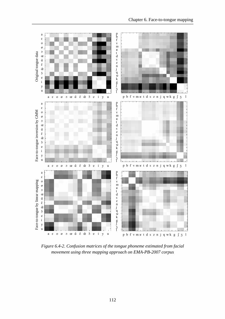
Chapter 6. Face-to-tongue mapping
112
Ori
gin
al to
ngu
e d
ata
a ɛ o ø ɔ œ ɑ ̃ɛ ̃œ̃ ɔ ̃e i y u
a ɛ o ø ɔ œ ɑ ̃ ɛ ̃ œ̃ ɔ ̃ e i y u
p b f v mʁ t d s z n j ɥ wk g ʃ ʒ l
p b f v m ʁ t d s z n j ɥ w k g ʃ ʒ l
Fac
e-to
-ton
gu
e in
vers
ion
by
GM
M a
ɛ o ø ɔ œ ɑ ̃ɛ ̃œ̃ ɔ ̃e i y u
a ɛ o ø ɔ œ ɑ ̃ ɛ ̃ œ̃ ɔ ̃ e i y u
p b f v mʁ t d s z n j ɥ wk g ʃ ʒ l
p b f v m ʁ t d s z n j ɥ w k g ʃ ʒ l
Fac
e-to
-to
ngu
e b
y lin
ear
map
pin
g a
ɛ o ø ɔ œ ɑ ̃ɛ ̃œ̃ ɔ ̃e i y u
a ɛ o ø ɔ œ ɑ ̃ ɛ ̃ œ̃ ɔ ̃ e i y u
p b f v mʁ t d s z n j ɥ wk g ʃ ʒ l
p b f v m ʁ t d s z n j ɥ w k g ʃ ʒ l
Figure 6.4-2. Confusion matrices of the tongue phoneme estimated from facial movement using three mapping approach on EMA-PB-2007 corpus
Chapter 6. Face-to-tongue mapping
113
6.5. Conclusion
We have revisited the Face-to-Tongue inversion problem in speech. Using a much larger corpus than previously in the literature (except for (Beskow et al., 2003)), we have assessed methods of different complexity and found that GMMs gave overall results better than HMMs, and that MLR did poorly. GMMs and HMMs can maintain the original phonetic class distribution, though with some centralisation effects those are still much stronger with MLR. Previous studies (Yehia et al., 1998; Jiang et al., 2002; Beskow et al., 2003) gave fairly good overall results, presumably because MLR copes well with limited material: we have shown that for larger corpuses, MLR gives poor results. As suggested by Jiang et al. (2002), more sophisticated context-sensitive techniques have improved the results fairly much. However, a detailed analysis has shown that, if the jaw / lips / tongue tip synergy helps recovering front high vowels and coronal consonants, the velars are not recovered at all. In conclusion, it is not possible to recover reliably tongue from face.

Chapter 7. Conclusions and perspectives
115
Chapter 7. Conclusions and perspectives
7.1. Conclusion
The focus of this thesis was the inversion of acoustic signals to articulatory movements based on statistical methods. These methods were implemented in a visual articulatory feedback system that automatically animates a 3D talking head from the speech sound. The visualisation of the articulatory feedback could be used in speech therapy and computer aided pronunciation.
Using electromagnetic articulography, we recorded two corpuses of parallel acoustic and articulatory data and used them to train and to test two statistical methods that we used to develop a robust acoustic-to-articulatory speech inversion system.
The first system developed is based on HMM models. The HMM-based method couples a speech synthesis system with a speech recogniser by jointly optimising a single statistical model for both acoustic and articulatory information using the multi-stream functionality supported by the HTK toolkit. The joint probability densities of the acoustic and articulatory features are modelled by context-dependent phone-sized HMM. Our experiments show that the minimum generation error (MGE) training of the articulatory stream improves the performance of the system, especially for the synthesis task. States tying and multi-Gaussians mixture were chosen in the acoustic stream for the output distribution in each state to provide a richer modelling capacity.
We also studied in this thesis another inversion method: we built GMM models that map directly the acoustic features to the articulatory ones. This method is inspired from the speech conversion system proposed by Toda and Shikano (2005). The MMSE criterion is used to predict the articulatory trajectories from the acoustic signal input, but the quality of the inversed articulation is however still insufficient for an articulatory feedback system. Articulatory prediction is then further improved by the use of the dynamic features in the MLE-based mapping.
We have benefited from the availability of articulatory data to study the relationships between face and tongue movements using HMMs and GMMs techniques compared to multi-linear regression (MLR) technique used in the literature. We found that GMMs gave overall results better than HMMs, and that MLR did poorly. Overall results were found not good enough to allow stating that it possible to recover reliably tongue from face. A detailed analysis showed for instance that the velars are not recovered at all.
In order to develop a multi-speaker system, we have used an MLLR adaptation technique to adapt in the acoustic domain the best HMMs to the voice of any new
Chapter 7. Conclusions and perspectives
116
speaker. The evaluation of this method has been done using an articulatory HMM-based phonetic recogniser. Recognition accuracies demonstrate the interest of the method.
Finally, we have developed a complete articulatory feedback demonstrator, which can work for any speaker with an adaptation procedure that requires a limited amount of acoustic data. A short video6 demonstrating the inversion of a few utterances spoken by speaker TH are available at http://www.gipsa-lab.inpg.fr/~atef.ben-youssef/recherches_en.html.
The proposed articulatory feedback system could be used in phonetic correction by displaying the target movement produced by the teacher and the erroneous movement produced by a learner, and highlighting the differences. Using text-to-articulatory synthesis, we can also display a phoneme sequence (i.e. VCV, words...) to show to the learner a correct articulation that (s)he can imitate.
7.2. Perspectives
Our experiments have also shown that the objective performance of our HMM-based speech inversion system is currently superior to the direct acoustic-to-articulatory mapping system based on the GMM models that we have implemented. Both systems could be improved by incorporating visual information as input and including this additional information more intimately in the optimisation process that will consider multimodal coherence between input and output parameters: lips are clearly visible and jaw is indirectly available in facial movements. The GMM-based system could be improved by considering other dimensionality reduction techniques such as Linear Discriminant Analysis (LDA) that are quite effective in HMM-based inversion (Tran et al., 2008).
Future work will also investigate different mapping techniques recently described in the literature, such as the low-delay implementation of the GMM-based mapping approach proposed by Muramatsu et al. (2008), which is based on the maximum likelihood estimation of the feature trajectories, and the approach based on trajectory HMM proposed by Zen et al. in (2010).
This HMM-based demonstrator does not run in real time at present, but a real time version of both voice conversion and inversion systems based on GMM-based method (i.e. unfortunately less accurate) has been developed by Hueber et al. (2011) on the same data. A real-time implementation of the HMM-based mapping approach is not as straightforward as for the GMM-based approach. As shown in equation (2.3-13), the HMM-based mapping is not a frame-by-frame process. The estimation of the
6 http://www.gipsa-lab.inpg.fr/~atef.ben-youssef/artis_demo.flv
Chapter 7. Conclusions and perspectives
117
articulatory features requires first the decoding of the most likely HMM state sequence (for the given sequence of acoustic vectors). This task, achieved by the Viterbi algorithm, is based on a backtracking procedure, and thus requires all observations from the first to the last to be available. In consequence, this algorithm is not well adapted to a real-time implementation. Different approaches have been proposed in the literature to decode HMM online. In (Seward, 2003), the Viterbi algorithm is applied on a sliding window of consecutive observations. The advantage of this method is that the additional delay it adds to the processing chain is constant (and equal to the length of the sliding window). However, this method does not guarantee that the sequence of successive “local” paths is identical to the optimal path, i.e. the path that would have been obtained if all the observations were taken into account. Bloit and Rodet (2008) proposed a short-time Viterbi algorithm, in which the Viterbi algorithm is applied on a sliding window of variable length. Under certain constraints on the HMM topology, the proposed algorithm guarantees that the successive decoded paths are identical to the optimal path. In this method, a constant maximum latency can also be obtained by forcing a suboptimal decoding when the window length exceeds a predefined threshold. We intend to implement a real-time version of the HMM-based mapping method in visual articulatory feedback system, based on the short time Viterbi algorithm (Bloit and Rodet, 2008).
Another important line of future work is to develop methods with generalisation capabilities for non-native speaker adaptation, as for instance done by (e.g. Ohkawa et al., 2009). Indeed, it is important that the inversion system can deal with L2 phonemes that the learner cannot produce at the beginning. It is therefore interesting to evaluate the generalisation capacity of both HMM and GMM systems to some kind of universal talking head. A preliminary experience on the generalisation capacity of the HMM-based technique was thus conducted. We assumed the case of an L1 having the five
vowels system /a i u ε o/ (e.g. Spanish or Japanese), and investigated the generalisation
to an L2 as French which has also vowels /e ø œ ɔ y/ that may be difficult to learn.
Using a set of HMMs consisting of the original set of trained (ctx-R) HMMs models,
where only the models corresponding to /a i u ε o/ were retained, and vowels /e ø œ ɔ
y/ were excluded (keeping on average over the 5 partitions about 271 used models from
the 327 original ones), we have inverted all acoustic signal of the test set (i.e. containing the sound corresponding to the eliminated models). Figure 7.2-1 shows that the global RMSE computed over the whole corpus increases from 1.65 mm when we inverse the acoustic signal using all trained models to 2.02 mm for the models trained only with the
five vowels /a i u ε o/ and all consonants. Moreover, when we calculate the RMSE by
phoneme, we find that the RMSE found using existing phoneme (trained) models is doubled compared to the eliminated phoneme models (from training).
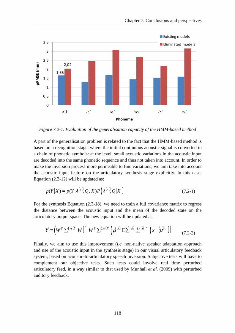
Chapter 7. Conclusions and perspectives
118
1,65
2,02
0
0,5
1
1,5
2
2,5
3
3,5
All /e/ /ø/ /œ/ /ɔ/ /y/
µR
MS
E (
mm
)
Phoneme
Existing models
Eliminated models
Figure 7.2-1. Evaluation of the generalisation capacity of the HMM-based method
A part of the generalisation problem is related to the fact that the HMM-based method is based on a recognition stage, where the initial continuous acoustic signal is converted in a chain of phonetic symbols: at the level, small acoustic variations in the acoustic input are decoded into the same phonetic sequence and thus not taken into account. In order to make the inversion process more permeable to fine variations, we aim take into account the acoustic input feature on the articulatory synthesis stage explicitly. In this case, Equation (2.3-12) will be updated as:
( ) ( )( )( ) ( , , ) ,y xp Y X p Y Q X P Q Xλ λ=
(7.2-1)
For the synthesis Equation (2.3-18), we need to train a full covariance matrix to regress the distance between the acoustic input and the mean of the decoded state on the articulatory output space. The new equation will be updated as:
( )( ) ( ) ( ) ( ) ( ) ( )( )( )1 1 11
ˆ yy yy y yx xx xT TY W W W xµ µ− − −−
= ∑ ∑ +∑ ∑ − (7.2-2)
Finally, we aim to use this improvement (i.e. non-native speaker adaptation approach and use of the acoustic input in the synthesis stage) in our visual articulatory feedback system, based on acoustic-to-articulatory speech inversion. Subjective tests will have to complement our objective tests. Such tests could involve real time perturbed articulatory feed, in a way similar to that used by Munhall et al. (2009) with perturbed auditory feedback.

Chapter 7. Conclusions and perspectives
119
This work will hopefully open possibilities for applications in the domain of speech therapy or CAPT (e.g. Engwall & Bälter (2007) or (Badin et al., 2008a)). The system we have developed (2010) is the most elaborate feedback system available at present.

Bibliography
121
Bibliography
Agelfors, E., Beskow, J., Karlsson, I., Kewley, J., Salvi, G., and Thomas, N. (2006). "User evaluation of the SYNFACE talking head telephone," Lecture Notes in Computer Science 4061, 579-586.
Al Moubayed, S., and Ananthakrishnan, G. (2010). "Acoustic-to-articulatory inversion based on local regression," in Proceedings of Interspeech 2010, edited by T. Kobayashi, K. Hirose, and S. Nakamura (Makuhari, Japan), pp. 937-940.
Ananthakrishnan, G., and Engwall, O. (2011). "Mapping between acoustic and articulatory gestures," Speech Communication 53, 567-589.
Atal, B. S., Chang, J. J., Mathews, M. V., and Tukey, J. W. (1978). "Inversion of articulatory-to-acoustic transformation in the vocal tract by a computer-sorting technique," Journal of the Acoustical Society of America 63, 1535-1555.
Badin, P., Elisei, F., Bailly, G., and Tarabalka, Y. (2008a). "An audiovisual talking head for augmented speech generation: models and animations based on a real speaker's articulatory data," in Vth Conference on Articulated Motion and Deformable Objects (AMDO 2008, LNCS 5098), edited by F. J. Perales, and R. B. Fisher (Springer Verlag, Berlin, Heidelberg, Germany), pp. 132–143.
Badin, P., and Fant, G. (1984). "Notes on vocal tract computation," Speech Transmission Laboratory - Quarterly Progress Status Report - Stockholm 2-3/1984, 53-108.
Badin, P., Tarabalka, Y., Elisei, F., and Bailly, G. (2008b). "Can you “read tongue movements”?," in Interspeech 2008 (Special Session: Talking Heads and Pronunciation Training) (Brisbane, Australia), pp. 2635-2638.
Badin, P., Tarabalka, Y., Elisei, F., and Bailly, G. (2010). "Can you 'read' tongue movements? Evaluation of the contribution of tongue display to speech understanding," Speech Communication 52, 493-503.
Bailly, G., and Badin, P. (2002). "Seeing tongue movements from outside," in 7th International Conference on Spoken Language Processing, ICSLP 2002 & Interspeech 2002 (Denver, Colorado, USA).
Bailly, G., Badin, P., Beautemps, D., and Elisei, F. (2010). "Speech technologies for augmented communication," in Computer Synthesized Speech Technologies: Tools for Aiding Impairment, edited by J. Mullennix, and S. Stern (IGI Global, Medical Information Science Reference), pp. 116-128.
Baum, L. E., and Petrie, T. (1966). "Statistical inference for probabilistic functions of finite state Markov chains.," Annals of Mathematical Statistics 37, 1554-1563.
Bibliography
122
Beautemps, D., Badin, P., and Bailly, G. (2001). "Linear degrees of freedom in speech production: Analysis of cineradio- and labio-film data and articulatory-acoustic modeling," Journal of the Acoustical Society of America 109, 2165-2180.
Ben Youssef, A., Badin, P., and Bailly, G. (2010). "Can tongue be recovered from face? The answer of data-driven statistical models," in Interspeech 2010 (11th Annual Conference of the International Speech Communication Association), edited by T. Kobayashi, K. Hirose, and S. Nakamura (Makuhari, Japan), pp. 2002-2005.
Ben Youssef, A., Badin, P., Bailly, G., and Heracleous, P. (2009). "Acoustic-to-articulatory inversion using speech recognition and trajectory formation based on phoneme hidden Markov models," in Proceedings of Interspeech 2009 (Brighton, UK), pp. 2255-2258.
Bernhardt, B. M., Bacsfalvi, P., Adler-Bock, M., Shimizu, R., Cheney, A., Giesbrecht, N., O'connell, M., Sirianni, J., and Radanov, B. (2008). "Ultrasound as visual feedback in speech habilitation: Exploring consultative use in rural British Columbia, Canada," Clinical Linguistics & Phonetics 22, 149-162.
Bernhardt, B. M., Gick, B., Bacsfalvi, P., and Adler-Bock, M. (2005). "Ultrasound in speech therapy with adolescents and adults," Clinical Linguistics & Phonetics 19, 605-617.
Bernhardt, B. M., Gick, B., Bacsfalvi, P., and Ashdown, J. (2003). "Speech habilitation of hard of hearing adolescents using electropalatography and ultrasound as evaluated by trained listeners," Clinical Linguistics & Phonetics 17, 199-216.
Beskow, J., Engwall, O., and Granström, B. (2003). "Resynthesis of facial and intraoral articulation from simultaneous measurements," in 15th International Congress of Phonetic Sciences, edited by M.-J. Solé, D. Recasens, and J. Romero (Barcelona, Spain), pp. 431-434.
Beskow, J., Karlsson, I., Kewley, J., and Salvi, G. (2004). "SYNFACE: A talking head telephone for the hearing-impaired," edited by K. Miesenberger, J. Klaus, W. Zagler, and D. Burger (Springer, Berlin, ALLEMAGNE), pp. 1178-1185.
Bloit, J., and Rodet, X. (2008). "Short-time Viterbi for online HMM decoding: Evaluation on a real-time phone recognition task," in Acoustics, Speech and Signal Processing, 2008. ICASSP 2008. IEEE International Conference on, pp. 2121-2124.
Blum, J. R. (1954). "Multidimensional Stochastic Approximation Methods," Annals of Mathematical Statistics 25, 737-744.
Boersma, P., and Weenink, D. (2005). "Praat: doing phonetics by computer (Version 4.3.14) [Computer program]. Retrieved May 26, 2005, from http://www.praat.org/."
Bozkurt, B., Ozturk, O., and Dutoit, T. (2003). "Text design for TTS speech corpus building using a modified greedy selection," in Proceedings of the Eurospeech’03 (Geneva, Switzerland), pp. 277--280.
Chun, D. M. (2007). "Come ride the wave: But where is it taking us?," Calico Journal 24, 239-252.
Bibliography
123
Cucchiarini, C., Neri, A., and Strik, H. (2009). "Oral proficiency training in Dutch L2: The contribution of ASR-based corrective feedback," Speech Communication 51, 853-863.
Demange, S., and Ouni, S. (2011). "Acoustic-to-articulatory inversion using an episodic memory," in International Conference on Acoustics, Speech and Signal Processing (ICASSP), edited by Ieee.
Engwall, O. (2000). "Are static MRI measurements representative of dynamic speech ? Results from a comparative study using MRI, EPG and EMA," in 6th International Conference on Spoken Language Processing, edited by B. Yuan, T. Huang, and X. Tang (Beijing, China), pp. 17-20.
Engwall, O. (2006). "Evaluation of speech inversion using an articulatory classifier.," in 7th International Seminar on Speech Production, ISSP7 (In Yehia, H., Demolin, D., & Laboissière, R. (Eds.), Ubatuba, Sao Paolo, Brazil. ), pp. 469-476.
Engwall, O. (2008). "Can audio-visual instructions help learners improve their articulation? — An ultrasound study of short term changes," in Proceedings of Interspeech 2008 (Brisbane, Australia), pp. 2631-2634.
Engwall, O., and Bälter, O. (2007). "Pronunciation feedback from real and virtual language teachers," Computer Assisted Language Learning 20, 235 - 262.
Engwall, O., and Beskow, J. (2003). "Resynthesis of 3D tongue movements from facial data," in Eurospeech 2003 (Geneva, Switzerland), pp. 2261-2264.
Fagel, S., and Madany, K. (2008). "A 3-D virtual head as a tool for speech therapy for children," in Proceedings of Interspeech 2008 (Brisbane, Australia), pp. 2643-2646.
Fowler, C. A., Brown, J. M., Sabadini, L., and Weihing, J. (2003). "Rapid access to speech gestures in perception: Evidence from choice and simple response time tasks," Journal of Memory & Language 49, 396-413.
François, H., and Boëffard, O. (2002). "The greedy algorithm and its application to the construction of a continuous speech database," in Proceedings of LREC-2002, pp. 1420-1426.
Furui, S. (1986). "Speaker-independent isolated word recognition using dynamic features of speech spectrum," IEEE transactions on acoustics, speech, and signal processing 34, 52-59.
Govokhina, O., Bailly, G., and Breton, G. (2007). "Learning optimal audiovisual phasing for a HMM-based control model for facial animation," in 6th ISCA Workshop on Speech Synthesis (Bonn, Germany).
Grauwinkel, K., Dewitt, B., and Fagel, S. (2007). "Visual information and redundancy conveyed by internal articulator dynamics in synthetic audiovisual speech," in Proceedings of Interspeech'2007 - Eurospeech - 9th European Conference on Speech Communication and Technology (Antwerp, Belgium), pp. 706-709.
Hiroya, S., and Honda, M. (2004). "Estimation of articulatory movements from speech acoustics using an HMM-based speech production model," IEEE Trans. Speech and Audio Processing 12, 175-185.
Bibliography
124
Hogden, J., Löfqvist, A., Gracco, V., Zlokarnik, I., Rubin, P. E., and Saltzman, E. L. (1996). "Accurate recovery of articulator positions from acoustics: new conclusions based on human data," Journal of the Acoustical Society of America 100, 1819-1834.
Hueber, T., Badin, P., Bailly, G., Ben Youssef, A., Elisei, F., Denby, B., and Chollet, G. (2011). "Statistical mapping between articulatory and acoustic data. Application to Silent Speech Interface and Visual Articulatory Feedback," in 1st International Workshop on Interactive Manipulation of Speech and Singing Synthesis [IM3S] (Vancouver, Canada).
Hueber, T., Chollet, G., Denby, B., and Stone, M. (2008). "Acquisition of ultrasound, video and acoustic speech data for a silent-speech interface application," in Proceedings of International Seminar on Speech Production (Strasbourg, France), pp. 365-369.
Iskarous, K., Goldstein, L. M., Whalen, D. H., Tiede, M. K., and Rubin, P. E. (2003). "CASY: The Haskins Configurable Articulatory Synthesizer," in 15th International Congress of Phonetic Sciences, edited by M.-J. Solé, D. Recasens, and J. Romero (Barcelona, Spain), pp. 185-188.
Jiang, J., Alwan, A. A., Keating, P. A., Auer, E. T., Jr, and Bernstein, J. (2002). "On the relationship between face movements, tongue movements, and speech acoustics," Special issue of EURASIP Journal on Applied Signal Provessing on joint audio-visual speech processing 2002, 1174-1188.
Joon, J. S. (2009). "A preliminary study of human motion based on actor physiques using motion capture," in Sixth International Conference on Computer Graphics, Imaging and Visualization, 2009. CGIV '09. (Tianjin), pp. 123 - 128.
Kain, A. (2001). "High Resolution Voice Transformation," in OGI School of Science & Engineering at Oregon Health & Science University, p. 115.
Kain, A., and Macon, M. W. (1998). "Spectral voice conversion for text-to-speech synthesis," in Acoustics, Speech and Signal Processing, 1998. Proceedings of the 1998 IEEE International Conference on, pp. 285-288 vol.281.
Karlsson, I. (2003). "The SYNFACE project – a status report," in Fonetik 2003 (Umeå University, Sweden), pp. 61-64.
Katsamanis, A., Papandreou, G., and Maragos, P. (2009). "Face Active Appearance Modeling and speech acoustic information to recover articulation," IEEE Transactions on Audio, Speech and Language Processing 17, 411-422.
Kiritani, S. (1986). "X-Ray microbeam method for measurement of articulatory dynamics-techniques and results," Speech Communication 5, 119-140.
Kjellström, H., and Engwall, O. (2009). "Audiovisual-to-articulatory inversion," Speech Communication 51, 195-209.
Kröger, B. J., Graf-Borttscheller, V., and Lowit, A. (2008). "Two- and three-dimensional visual articulatory models for pronunciation training and for treatment of speech disorders," in Proceedings of Interspeech 2008 (Brisbane, Australia), pp. 2639-2642.
Bibliography
125
Lachambre, H., Koenig, L., and André-Obrecht, R. (2011). "Articulatory Parameter Generation using Unsupervised Hidden Markov Model," in European Signal Processing Conference (EUSIPCO) (Barcelona, Spain).
Lammert, A., Ellis, D. P. W., and Divenyi, P. (2008). "Data-driven articulatory inversion incorporating articulator priors," in Proceedings of Interspeech 2008 (Brisbane, Australia), pp. 29-34.
Lammert, A., Goldstein, L., and Iskarous, K. (2010). "Locally-Weighted Regression for Estimating the Forward Kinematics of a Geometric Vocal Tract Model," in Interspeech 2010, edited by T. Kobayasih, H. keikichi, and S. Nakamura (Makuhari, Japan), pp. 1604-1607.
Laprie, Y., and Ouni, S. (2002). "Introduction of constraints in an acoustic-to-articulatory inversion," in 7th International Conference on Spoken Language Processing - ICSLP 2002 (none).
Leggetter, C., and Woodland, P. (1995). "Maximum likelihood linear regression for speaker adaptation of continuous density hidden Markov models," Computer, Speech and Language 9, 171-185.
Levitt, J. S., and Katz, W. F. (2010). "The Effects of EMA-Based Augmented Visual Feedback on the English Speakers' Acquisition of the Japanese Flap: A Perceptual Study," in Interspeech 2010 (11th Annual Conference of the International Speech Communication Association), edited by T. Kobayashi, K. Hirose, and S. Nakamura (Makuhari, Japan), pp. 1862-1865.
Ling, Z.-H., Richmond, K., and Yamagishi, J. (2010). "An Analysis of HMM-based prediction of articulatory movements," Speech Communication 52, 834-846.
Maeda, S. (1988). "Improved articulatory models," Journal of the Acoustical Society of America 84, S146.
Maeda, S. (1990). "Compensatory articulation during speech: Evidence from the analysis and synthesis of vocal-tract shapes using an articulatory model," in Speech Production and Modelling, edited by W. J. Hardcastle, and A. Marchal (Academic Publishers, Kluwer), pp. 131-149.
Massaro, D. W., Bigler, S., Chen, T., Perlman, M., and Ouni, S. (2008). "Pronunciation training: the role of eye and ear," in Proceedings of Interspeech 2008 (Brisbane, Australia), pp. 2623-2626.
Massaro, D. W., and Light, J. (2004). "Using visible speech to train perception and production of speech for individuals with hearing loss," Journal of Speech, Language, and Hearing Research 47, 304-320.
Masuko, T., Tokuda, K., Kobayashi, T., and Imai, S. (1996). "Speech synthesis using HMMs with dynamic features," in Proceedings of the Acoustics, Speech, and Signal Processing, 1996. on Conference Proceedings., 1996 IEEE International Conference - Volume 01 (IEEE Computer Society), pp. 389-392.
Mawass, K., Badin, P., and Bailly, G. (2000). "Synthesis of French fricatives by audio-video to articulatory inversion," Acta Acustica 86, 136-146.
Menin-Sicard, A., and Sicard, E. (2006). "Evaluation et rééducation de la voix et de la parole avec Vocalab," Glossa 88, 62-76.
Bibliography
126
Menzel, W., Herron, D., Morton, R., Pezzotta, D., Bonaventura, P., and Howarth, P. (2001). "Interactive pronunciation training," ReCALL 13, 67-78.
Mermelstein, P. (1973). "Articulatory model for study of speech production," Journal of the Acoustical Society of America 53, 1070-1082.
Montgomery, D. (1981). "Do dyslexics have difficulty accessing articulatory information?," Psychological Research 43.
Munhall, K. G., MacDonald, E. N., Byrne, S. K., and Johnsrude, I. (2009). "Talkers alter vowel production in response to real-time formant perturbation even when instructed not to compensate," The Journal of the Acoustical Society of America 125(1), 384-390.
Muramatsu, T., Ohtani, Y., Toda, T., Saruwatari, H., and Shikano, K. (2008). "Low-delay voice conversion based on maximum likelihood estimation of spectral parameter trajectory," in Proceedings of Interspeech 2008, pp. 1076-1079.
Neri, A., Cucchiarini, C., and Strik, H. (2002). "Feedback in computer assisted pronunciation training: technology push or demand pull?," in ICSLP-2002 (Denver, Co, USA), pp. 1209-1212.
Odisio, M., Bailly, G., and Elisie, F. (2004). "Shape and appearance models of talking faces for model-based tracking.," Speech Communication 44, 63-82.
Ohkawa, Y., Suzuki, M., Ogasawara, H., Ito, A., and Makino, S. (2009). "A speaker adaptation method for non-native speech using learners' native utterances for computer-assisted language learning systems," Speech Communication 51, 875-882.
Okadome, T., Kaburagi, T., and Honda, M. (1999). "Articulatory movement formation by kinematic triphone model," in IEEE International Conference on Systems, Man, and Cybernetics, IEEE SMC '99 (Tokyo, Japan), pp. 469-474.
Ouni, S., and Laprie, Y. (1999). "Design of hypercube codebooks for the acoustic-to-articulatory inversion respecting the non-linearities of the articulatory-to-acoustic mapping," in 6th EuroSpeech Conference (Budapest, Hungary), pp. 141-144.
Ouni, S., and Laprie, Y. (2005). "Modeling the articulatory space using a hypercube codebook for acoustic-to-articulatory inversion," Journal of the Acoustical Society of America 118, 444-460.
Panchapagesan, S., and Alwan, A. (2011). "A study of acoustic-to-articulatory inversion of speech by analysis-by-synthesis using chain matrices and the Maeda articulatory model," The Journal of the Acoustical Society of America 129, 2144-2162.
Peckels, J., and Rossi, M. (1973). "Le test de diagnostic par paires minimales," Revue d'Acoustique 27, 245-262.
Potard, B. (2008). "Inversion acoustique-articulatoire avec contraintes," in LORIA at Nancy 1 ( Nancy 1, Nancy), p. 156.
Bibliography
127
Qin, C., and Carreira-Perpiñán, M. A. (2007). "A comparison of acoustic features for articulatory inversion," in Proceedings of Interspeech 2007 (Antwerp, Belgium), pp. 2469-2472.
Rabiner, L. R. (1989). "A tutorial on hidden Markov models and selected applications in speech recognition," Proceedings of the IEEE 77, 257-286.
Richmond, K. (2002). "Estimating articulatory parameters from the acoustic speech signal," in The Centre for Speech Technology Research (Edinburgh University, Edinburgh).
Richmond, K. (2006). "A Trajectory Mixture Density Network for the Acoustic-Articulatory Inversion Mapping," in Interspeech 2006 (Pittsburgh, USA), pp. 577-580.
Richmond, K. (2007). "Trajectory mixture density networks with multiple mixtures for acoustic-articulatory inversion," in Advances in Nonlinear Speech Processing (Lecture Notes in Computer Science 4885) (Springer Verlag, Berlin, Heidelberg, Germany), pp. 263-272.
Richmond, K. (2009). "Preliminary Inversion Mapping Results with a New EMA Corpus," in Proceedings of Interspeech 2009 (Brighton, UK), pp. 2835-2838.
Richmond, K., King, S., and Taylor, P. (2003). "Modelling the uncertainty in recovering articulation from acoustics," Computer Speech and Language 17, 153-172.
Ridouane, R. (2006). Investigating speech production A review of some techniques.
Rubin, P. E., Saltzman, E. L., Goldstein, L., McGowan, R. S., Tiede, M. K., and Browman, C. P. (1996). "CASY and extensions to the task-dynamic model," in 4th Speech Production Seminar - 1st ESCA Tutorial and Research Workshop on Speech Production Modeling: from Control Strategies to Acoustics (Autrans, France), pp. 125-128.
Russell, G. O. (1928). "The vowel, its psychological mechanism, as shown by x-ray," in Columbus OH: Ohio State University Press.
Saino, K., Zen, H., Nankaku, Y., Lee, A., and Tokuda, K. (2006). "An HMM-based singing voice synthesis system," in Proceedings of Interspeech 2006 (ISCA, Pittsburgh, PA, USA), pp. 1141-1144.
Schroeter, J., and Sondhi, M. M. (1994). "Techniques for estimating vocal-tract shapes from the speech signal," IEEE Transactions on Speech and Audio Processing, 2, 133-150.
Seward, A. (2003). "Low-Latency Incremental Speech Transcription in the Synface Project," in Proceedings of the European Conference on Speech Communication and Technology (Eurospeech), Geneva, Switzerland, 2003 : vol 2, pp. 1141-1144.
Smola, A., and Schölkopf, B. (2004). "A tutorial on support vector regression," Statistics and Computing 14, 199-222.
Stetson, R. H. (1928). "Motor phonetics. A study of speech movements in action," Archives Néerlandaises de Phonétique Expérimentale 3, 216.
Bibliography
128
Stone, M. (1990). "A three-dimensional model of tongue movement based on ultrasound and x-ray microbeam data," Journal of the Acoustical Society of America 87, 2207-2217.
Stone, M., Sonies, B., Shawker, T., Weiss, G., and Nadel, L. (1983). "Analysis of real-time ultrasound images of tongue configuration using a grid-digitizing system," Journal of Phonetics 11, 207–218.
Stone, M., Stock, G., Bunin, K., Kumar, K., Epstein, M. A., Kambhamettu, C., Li, M., Parthasarathy, V., and Prince, J. (2007). "Comparison of speech production in upright and supine position," The Journal of the Acoustical Society of America 122.
Stylianou, Y., Cappé, O., and Moulines, E. (1998). "Continuous probabilistic transform for voice conversion," IEEE Transactions on Speech and Audio Processing 6, 131-142.
Sumby, W. H., and Pollack, I. (1954). "Visual contribution to speech intelligibility in noise," Journal of the Acoustical Society of America 26, 212-215.
Tepperman, Joseph, Narayanan, and Shrikanth (2008). "Using Articulatory Representations to Detect Segmental Errors in Nonnative Pronunciation," IEEE Transactions on Audio, Speech and Language Processing 16(1), 8-22.
Thomas, E. M., and Sénéchal, M. (1998). "Articulation and phoneme awareness of 3-year-old children," Applied Psycholinguistics 19, 363-391.
Tiede, M. K., Masaki, S., and Vatikiotis-Bateson, E. (2000). "Contrasts in speech articulation observed in sitting and supine conditions," in 5th Seminar on Speech Production: Models and Data & CREST Workshop on Models of Speech Production: Motor Planning and Articulatory Modelling (Kloster Seeon, Germany), pp. 25-28.
Toda, T., Black, A. W., and Tokuda, K. (2004a). "Acoustic-to-Articulatory Inversion Mapping with Gaussian Mixture Model," in Proceedings of Interspeech 2004 (Jeju, Korea), pp. 1129-1132.
Toda, T., Black, A. W., and Tokuda, K. (2004b). "Mapping from articulatory movements to vocal tract spectrum with Gaussian mixture model for articulatory speech synthesis," in International Speech Synthesis Workshop (Pittsburgh, PA), pp. 31-36.
Toda, T., Black, A. W., and Tokuda, K. (2005). "Spectral conversion based on Maximum Likelihood Estimation considering Global Variance of converted parameter," in IEEE International Conference on Acoustics, Speech, and Signal Processing, pp. 9-12.
Toda, T., Black, A. W., and Tokuda, K. (2008). "Statistical mapping between articulatory movements and acoustic spectrum using a Gaussian mixture model," Speech Communication 50, 215-227.
Toda, T., and Shikano, K. (2005). "NAM-to-speech conversion with Gaussian Mixture Models," in Interspeech'2005 - Eurospeech - 9th European Conference on Speech Communication and Technology (Lisbon, Portugal), pp. 1957-1960.
Bibliography
129
Tokuda, K., Masuko, T., Yamada, T., Kobayashi, T., and Imai, S. (1995). "An algorithm for speech parameter generation from continuous mixture HMMs with dynamic features," in 4th EuroSpeech Conference, edited by J. M. Pardo, E. Enríquez, J. Ortega, J. Ferreiros, J. Macías, and F. J. Valverde (Gráficas Brens, Madrid, Spain), pp. 757-760.
Tokuda, K., Yoshimura, T., Masuko, T., Kobayashi, T., and Kitamura, T. (2000). "Speech parameter generation algorithms for HMM-based speech synthesis," in IEEE International Conference on Acoustics, Speech, and Signal Processing (Istanbul, Turkey), pp. 1315-1318.
Toutios, A., and Margaritis, K. (2005a). "Mapping the Speech Signal onto Electromagnetic Articulography Trajectories Using Support Vector Regression," in Text, Speech and Dialogue, edited by V. Matoušek, P. Mautner, and T. Pavelka (Springer, Berlin / Heidelberg), pp. 318-325.
Toutios, A., and Margaritis, K. (2005b). "A support vector approach to the acoustic-to-articulatory mapping," in Proceedings of Interspeech 2005 (Lisbon, Portugal), pp. 3221-3224.
Tran, V.-A. (2010). "Silent Communication : whispered speech-to-clear speech conversion," in GIPSA-Lab at Grenoble Institute of Technology, p. 161.
Tran, V.-A., Bailly, G., Loevenbruck, H., and Jutten, C. (2008). "Improvement to a NAM captured whisper-to-speech system," in Interspeech (Brisbane, Australia), pp. 1465-1468.
Tye-Murray, N., Kirk, K. I., and Schum, L. (1993). "Making typically obscured articulatory activity available to speechreaders by means of videofluoroscopy," NCVS Status and Progress Report 4, 41-63.
Van Santen, J. P. H., and Buchsbaum, A. L. (1997). "Methods for optimal text selection," in 5th EuroSpeech Conference (Rhodos, Greece), pp. 553-556.
Wik, P., and Engwall, O. (2008). "Can visualization of internal articulators support speech perception?," in Interspeech 2008 (Brisbane, Australia), pp. 2627-2630.
Wrench, A., Gibbon, F., McNeill, A. M., and Wood, S. (2002). "An EPG therapy protocol for remediation and assessment of articulation disorders," in ICSLP-2002, pp. 965-968.
Wu, Y.-J., Wu, G., and Wang, R. H. (2006). "Minimum generation error criterion for tree-based clustering of context dependent HMMs," in Proceedings of Interspeech 2006 (Pittsburgh, USA), pp. 2046-2049.
Wu, Y. J., Zen, H., Nankaku, Y., and Tokuda, K. (2008). "Minimum generation error criterion considering global/local variance for HMM-based speech synthesis," in ICASSP (Las Vegas, NE, USA), pp. 4621-4624.
Yehia, H. C., Rubin, P. E., and Vatikiotis-Bateson, E. (1998). "Quantitative association of vocal-tract and facial behavior," Speech Communication 26, 23-43.
Young, S., Evermann, G., Gales, M., Hain, T., Kershaw, D., Liu, X. A., Moore, G., Odell, J., Ollason, D., Povey, D., Valtchev, V., and Woodland, P. (2009). "The HTK Book (for HTK Version 3.4). Revised for HTK Version 3.4 March 2009."
Bibliography
130
Zen, H., Masuko, T., Tokuda, K., Yoshimura, T., Kobayasih, T., and Kitamura, T. (2007a). "State Duration Modeling for HMM-Based Speech Synthesis," IEICE - Trans. Inf. Syst. E90-D, 692-693.
Zen, H., Nankaku, Y., and Tokuda, K. (2010). "Continuous Stochastic Feature Mapping Based on Trajectory HMMs," Audio, Speech, and Language Processing, IEEE Transactions on 19, 417-430.
Zen, H., Nankaku, Y., and Tokuda, K. (2011). "Continuous Stochastic Feature Mapping Based on Trajectory HMMs," Audio, Speech, and Language Processing, IEEE Transactions on 19, 417-430.
Zen, H., Nose, T., Yamagishi, J., Sako, S., Masuko, T., Black, A., and Tokuda, K. (2007b). "The HMM-based speech synthesis system (HTS) version 2.0," in Proceedings of the 6th ISCA Workshop on Speech Synthesis (SSW6) (Bonn, Germany), pp. 294-299.
Zen, H., Tokuda, K., and Black, A. W. (2009). "Statistical parametric speech synthesis," Speech Communication 51, 1039-1064.
Zen, H., Tokuda, K., and Kitamura, T. (2004). "An introduction of trajectory model into HMM-based speech synthesis," in Fifth ISCA ITRW on Speech Synthesis (SSW5) (Pittsburgh, PA, USA), pp. 191-196.
Zhang, L. (2009). "Modelling Speech Dynamics with Trajectory-HMMs.," in The Centre for Speech Technology Research (School of Informatics, Edinburgh University, Edinburgh), p. 135.
Zhang, L., and Renals, S. (2008). "Acoustic-articulatory modeling with the trajectory HMM," IEEE Signal Processing Letters 15, 245-248.
Résumé en français de la thèse
131
Appendix A
Résumé en français de la thèse
Cette annexe contient un résumé détaillé en français du travail effectué dans cette thèse.
1. Introduction
Il existe des preuves solides montrant que les systèmes cognitifs et sensori-moteurs sont largement couplés et que le liage intuitif entre gestes articulatoires et leurs conséquences audiovisuelles peut être exploité par le système perceptif: les articulateurs visibles, tel que la mâchoire et les lèvres, améliorent l'intelligibilité de la parole (Sumby and Pollack, 1954), l'imitation est plus rapide lorsque les gestes articulatoires sont visibles (Fowler et al., 2003), et la vision des articulateurs cachés, comme la langue et le velum, augmente aussi l'intelligibilité de la parole (Badin et al., 2010).
Il apparaît donc que la parole augmentée, c'est-à-dire la parole audio complétée par d’autres signaux (vidéo, affichage des articulateurs cachés tels que la langue ou le velum à l'aide d'une tête parlante virtuelle, gestes de la main utilisés dans le langage parlé complété par les personnes malentendantes, etc.) offre des potentialités très intéressantes dans les situations de communication où le signal audio lui-même est dégradé (environnement bruité, déficience auditive, etc.), ou dans le domaine de la rééducation de la parole (orthophonie, correction phonétique, etc.)
L'inversion acoustico-articulatoire, c'est-à-dire la récupération des gestes articulatoires à partir du signal audio ou audio-visuel, est encore actuellement un problème difficile. La principale difficulté consiste en l’absence de correspondance directe univoque entre le signal acoustique et le geste articulatoire : Atal et al. (1978) ont montré qu’un grand nombre de formes du conduit vocal peuvent produire le même signal acoustique. L’utilisation de contraintes (contextuelles, linguistiques, etc.) à la fois suffisamment restrictives et réalistes d'un point de vue phonétique, peut permettre de sélectionner les solutions optimales.
L'objectif global de cette thèse est donc de développer des outils d'inversion acoustico-articulatoire et de construire un système pouvant produire de la parole augmentée à partir du signal sonore seul. Plus précisément, nous avons tenté de construire un
Résumé en français de la thèse
132
système de retour articulatoire visuel qui peut être utilisé pour l’apprentissage de la prononciation assistée par ordinateur dans le cas de langues secondes, ou pour la réhabilitation des troubles de la parole.
Ce qui suit est un résumé de nos contributions.
Note : projet ARTIS. Le travail présenté dans cette thèse a constitué une contribution importante au projet ANR-08-EMER-001-02 ARTIS en collaboration entre le GIPSA-lab, le LORIA, l'ENST-Paris et l’IRIT. L'objectif principal de ce projet de recherche est de fournir de la parole augmentée par les articulateurs visibles et cachés au moyen d'une tête parlante à partir du signal sonore de parole seul ou avec les images vidéo du visage de du locuteur.
2. Retour articulatoire visuel
Bien que la contribution de la vision des articulateurs externes (lèvres, visage) à la perception de la parole soit largement établie, les études sur la contribution de la vision des articulateurs cachés tels que la langue ou le vélum à la perception de la parole sont extrêmement peu nombreuses (cf. Badin et al., 2010).
2.1. Retour articulatoire visuel pour la correction phonétique
La correction phonétique intervient dans deux domaines : l'apprentissage des langues étrangères et la réhabilitation du langage. Dans ces deux domaines, les chercheurs ont tenté de fournir aux apprenants/patients divers signaux portant de l’information complémentaire au signal audio et liés à leur production de parole.
Des recherches ont montré que les technologies de retour visuel, acoustique ou articulatoire, peuvent être des outils efficaces pour la réhabilitation du langage (Bernhardt et al., 2005; 2008). Les informations acoustiques peuvent être affichées comme des formes d'onde, des trajectoires temporelles de l'intensité ou de la fréquence fondamentale, ou encore des spectrogrammes (Neri et al., 2002; Menin-Sicard and Sicard, 2006). Pendant les sessions cliniques conduites par Wrench et al. (2002), le patient pouvait utiliser le retour visuel des contacts langue - palais fournis par Électro PalatoGraphie (EPG) pour établir le placement vélaire / alvéolaire pour les différentes cibles phonétiques. Bernhardt et al. (2005) ont utilisé l’imagerie ultrasonique de la langue pour afficher la forme de la langue sur un écran d’ordinateur et permettre aux patients de comparer leurs propres productions avec les productions cibles proposées par les orthophonistes. Globalement, la plupart des études semblent montrer que le retour articulatoire visuel facilite la réhabilitation de langage par visualisation de la forme et du mouvement de la langue (Bernhardt et al., 2003).
A l’opposé de l'orthophonie, la plupart de la littérature sur l’apprentissage de la prononciation assisté par ordinateur semble traiter un retour visuel qui n'implique pas d'informations explicites articulatoires. La reconnaissance automatique de la parole est
Résumé en français de la thèse
133
ainsi souvent utilisée pour localiser les erreurs, et même effectuer des analyses en termes de substitutions de phone, insertions ou suppressions. Bien que les systèmes de reconnaissance vocale soient de plus en plus précis et flexibles, et aient permis des progrès dans l’apprentissage de la prononciation assisté par ordinateur (Chun, 2007), (Cucchiarini et al., 2009), il semble intéressant d'explorer les potentialités du retour articulatoire visuel.
2.2. Tête parlante et parole augmentée
Comme mentionné précédemment, l'objectif du présent travail est de mettre en œuvre et tester un système de retour articulatoire visuel pour l’apprentissage de la prononciation assisté par ordinateur et pour la réhabilitation du langage. Une approche par modélisation offre une alternative intéressante aux dispositifs tels que l’EPG ou l’imagerie ultrasonique: la tête parlante virtuelle développée dans notre département comme assemblage de modèles articulatoires tridimensionnels des organes de la parole d’un même locuteur construits à partir de données statiques, telles que des images obtenues par résonance magnétique (IRM), peut être contrôlée au cours du temps par des dispositifs de capture de mouvement tels que l’articulographe électromagnétique (Electromagnetic Articulography, EMA) qui fournit les trajectoires de bobines attachées aux articulateurs à une fréquence d'échantillonnage suffisamment élevée (Badin et al., 2008a). Cette tête parlante offre des possibilités de parole augmentée en permettant un affichage visuel des articulateurs visibles et non visibles beaucoup plus complet que l'EPG ou l’échographie (cf. Badin et al. (2008a; 2010) pour une description détaillée).
2.3. Système de retour articulatoire visuel
Notre système de retour articulatoire visuel se concentre sur un paradigme spécifique: un retour articulatoire au moyen de la tête parlante d’un « enseignant » censé être bilingue en deux langues L1 et L2, dans le but d’aider un apprenant dont la langue maternelle est L1 et qui apprend la langue étrangère L2.
Dans ce cadre général, des paradigmes avec plusieurs niveaux de complexité croissante pourraient être envisagés :
Le premier niveau consiste à fournir à l'apprenant un retour articulatoire en utilisant son propre modèle articulatoire, dans sa langue maternelle L1. Cela peut être fait de la même manière que pour l'enseignant dans les deux langues L1 et L2.
Au deuxième niveau, le modèle articulatoire de l'enseignant développé dans la langue L1 est utilisé pour fournir un retour articulatoire à l'apprenant qui aura comme tâche de « l’imiter » dans sa langue maternelle L1.
Un niveau encore plus élaboré consiste à utiliser le modèle articulatoire de l'apprenant développé dans L1 pour fournir un retour à l'apprenant dans la langue étrangère L2. Être
Résumé en français de la thèse
134
capable de réaliser cela dépend des capacités des méthodes d'inversion entraînées dans une langue à opérer sur une autre langue.
3. Inversion de la parole par des méthodes statistiques
3.1. Revue de la littérature
L’inversion en parole a été longtemps basée sur le paradigme d’analyse par la synthèse. Mais depuis une décade, des techniques d’apprentissage plus sophistiquées sont apparues, grâce à la disponibilité de corpus importants de données articulatoires et acoustiques produites par des dispositifs tels que l’articulographe électromagnétique (EMA) ou les dispositifs de suivi de marqueurs basés sur la vidéo classique ou infrarouge.
Dans la littérature récente, on peut trouver un certain nombre de modèles statistiques de production et d’inversion de parole : modèles de Markov cachés (Hidden Markov Models, HMMs) (Hiroya and Honda, 2004), (Zhang and Renals, 2008; Zhang, 2009), (Ling et al., 2010), modèles de mélanges de Gaussiennes (Gaussian Mixture Models, GMMs) (Toda et al., 2008), (Zen et al., 2011), réseaux de neurones artificiels (Artificial Neural Networks, ANNs) (Richmond, 2007), machines à vecteurs de support (Support Vector Machines, SVMs) (Toutios and Margaritis, 2005a; Toutios and Margaritis, 2005b). La différence structurelle entre les HMMs et les autres modèles (GMMs, ANNs, SVMs) réside dans le fait que les HMMs utilisent explicitement des informations phonétiques et des contraintes phonotactiques et linguistiques, tandis que les autres modèles agrègent simplement le comportement multimodal de segments de parole similaires.
Hiroya & Honda (2004) ont développé une méthode qui estime les mouvements articulatoires à partir du son à l’aide d’un modèle de production de parole basé sur les HMMs. Le modèle de chaque phone comprend un HMM des paramètres articulatoires dépendant du contexte et un associateur linéaire qui transforme les paramètres articulatoires en spectre de parole pour chacun des états du HMM. Les modèles sont construits à partir d’observations acoustiques et articulatoires simultanées acquises par EMA. La séquence des états HMM correspondant à une phrase est déterminée en cherchant le maximum de vraisemblance de la séquence de spectres de parole produits par les modèles de production. Les paramètres articulatoires sont ensuite déterminés en cherchant le maximum de l’estimation a posteriori des paramètres articulatoires pour un spectre de parole donné et la séquence des états HMM. L’erreur racine de l’erreur quadratique moyenne (Root Mean Square Error, RMSE) obtenue est de 1,73 mm.
Toda et al. (2008) ont décrit une approche statistique à la fois pour la transformation articulatoire vers acoustique et la transformation inverse acoustique vers articulatoire sans information phonétique. Ils modélisent la densité de probabilité conjointe des trames acoustiques et articulatoires en contexte par un modèle GMM entraîné sur une
Résumé en français de la thèse
135
base de données parallèles acoustiques et articulatoires. Ils utilisent deux techniques différentes pour établir la transformation GMM. Avec un critère d’erreur quadratique moyenne minimum (Minimum Mean Square Error, MMSE) sur une fenêtre acoustique de 11 trames et 32 composantes pour le GMM, ils obtiennent des erreurs RMSE d’inversion de 1,61 mm pour une locutrice, et de 1,53 mm pour un locuteur. L’utilisation d’une méthode de maximum de vraisemblance (Maximum Likelihood Estimation, MLE) avec 64 composantes gaussiennes, réduit les erreurs à 1,45 mm pour la locutrice, et à 1,36 mm pour le locuteur.
Les études décrites ci-dessus ne permettent pas de déterminer la méthode d’inversion optimale, puisque les données, les locuteurs et les langues ne sont pas comparables. En outre, les corpus ainsi que les conditions d’apprentissage et de test ne sont pas non plus comparables.
3.2. Inversion par des modèles de Markov cachés
Les procédures d’apprentissage et de test ont été réalisées avec les boîtes à outils HTK (Young et al., 2009) et HTS (Zen et al 2007). . Nous avons utilisé des modèles HMM gauche-droite à trois états, avec une matrice de covariance diagonale. Les vecteurs de traits acoustiques et articulatoires sont considérés comme deux flux dans la procédure multi-flux de HTK. Les modèles HMMs obtenus sont ensuite séparés en HMMs articulatoires et HMMs acoustiques. Les HMMs acoustiques sont représentés par 8 gaussiennes par état tandis que les HMMs articulatoires contiennent une seule gaussienne par état. Les états ayant des distributions statistiques proches sont liés, c’est-à-dire regroupés pour permettre l’estimation des paramètres sur un plus grand nombre d’occurrences. Pour l’apprentissage, les paramètres du modèle HMM acoustique sont entraînés suivant le critère de maximum de vraisemblance (Maximum Likelihood, ML). En complément, nous avons implémenté le critère de minimisation de l’erreur générée (Minimum Generation Error, MGE) (Wu et al., 2006; Wu et al., 2008) pour ré-estimer les paramètres des HMMs articulatoires.
Différentes variantes ont été testées: phonèmes sans contexte (no-ctx), avec contexte gauche (L-ctx) ou droit (ctx-R), et avec contextes gauche et droit (L-ctx-R). Une méthode de regroupement hiérarchique, basée sur la matrice des distances de Mahalanobis entre les coordonnées des bobines pour chaque paire de phonèmes, a
permis de définir six classes cohérentes pour les contextes vocaliques ([a ɛ ɛ ̃| ø œ œ̃ | e
i | y | u | o ɔ ɑ ̃ɔ]̃) et dix classes pour les contextes consonantiques ([p b m | f v | ʁ | ʃ ʒ |
l | t d s z n | j | ɥ | k g | w]). Le schwa et les pauses courtes ou longues ([ə _ __]) ne sont
pas pris en compte comme contextes.
Un modèle de langage bi-gramme considérant les séquences de phones en contexte est appris sur la transcription phonétique du journal Le Monde (année 2003). L’inversion est réalisée en deux étapes : la première effectue une reconnaissance phonémique basée
Résumé en français de la thèse
136
sur les HMMs acoustiques, et fournit la séquence des allophones reconnus, ainsi que la durée de chaque état. Une procédure d’héritage permet de remplacer un HMM en contexte manquant dans le corpus d’apprentissage par le HMM le plus proche (Ben Youssef et al., 2009). La seconde étape effectue la synthèse des trajectoires articulatoires à partir de ces informations à l’aide de la procédure de formation de trajectoire proposée par Zen et al. (2004).
3.3. Inversion par des modèles de mélange de Gaussiennes
Nous avons mis en œuvre une mise en correspondance basée sur les GMMs en utilisant le critère de minimum de l’erreur quadratique moyenne (MMSE), souvent utilisé pour la conversion de voix. En outre, afin d’améliorer la précision de l’inversion, nous avons ajouté une étape d’optimisation basée sur l’estimation du maximum de vraisemblance (MLE) (Toda et al., 2008). Les trajectoires des paramètres cibles ayant les propriétés statiques et dynamiques adéquates sont déterminées en combinant les estimations locales de la moyenne et de la variance pour chaque trame p(t) et ses dérivées ∆p(t) par
la relation explicite entre les paramètres statiques et dynamiques (p. ex. ∆p(t) = p(t) – p(t-1)). A chaque trame articulatoire, le contexte est construit en concaténant les vecteurs acoustiques de plusieurs trames autour de la trame courante, afin de prendre en compte le contexte acoustique. De 9 à 13 vecteurs acoustiques sont prélevés de manière équirépartie dans une zone temporelle contextuelle de taille variable, et réduits à NACP = 24 composantes par Analyse en Composantes Principales (Toda et al., 2008; Tran et al., 2008). Pour chaque trame, le vecteur de traits est la concaténation du vecteur articulatoire DEMA des coordonnées (x, y) des bobines EMA et de leurs dérivées temporelles, avec le vecteur acoustique de NACP composantes. Nous avons fait varier le nombre de composantes gaussiennes de 16 à 128 et la zone contextuelle d’une taille phonémique (~90 ms) à une taille plus grande (~130 ms). Chaque gaussienne est représentée par une matrice de covariance pleine (48×48), un vecteur de moyennes (48) et son coefficient de pondération.
4. Données acoustiques et articulatoires
Alors que les signaux acoustiques de la parole peuvent être enregistrés simplement par un microphone, plusieurs méthodes ont été proposées au fil des années pour mesurer la forme du conduit vocal et le mouvement des articulateurs : cinéradiographie (Russell, 1928), microfaisceaux de rayons X (Kiritani, 1986), Imagerie par Résonance Magnétique (IRM), échographie ultrasonore (Stone et al., 1983; Stone, 1990), (Hueber et al., 2008), par vidéo (Badin et al., 2002) ou articulographe électromagnétique (Perkell et al., 1992).
Dans cette thèse, trois corpus enregistrés à l’aide d’un articulographe EMA ont été utilisés : deux corpus français enregistrés par le même locuteur et un corpus anglais MOCHA-TIMIT enregistré par une locutrice.
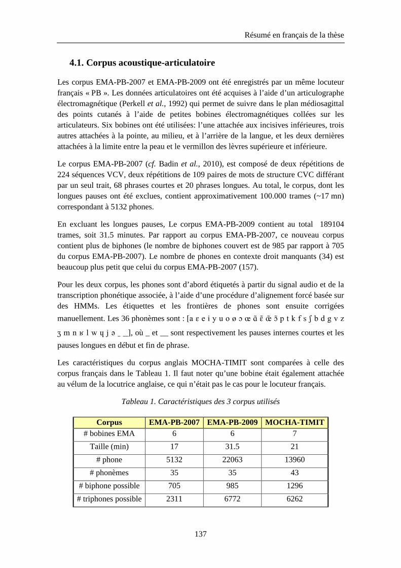
Résumé en français de la thèse
137
4.1. Corpus acoustique-articulatoire
Les corpus EMA-PB-2007 et EMA-PB-2009 ont été enregistrés par un même locuteur français « PB ». Les données articulatoires ont été acquises à l’aide d’un articulographe électromagnétique (Perkell et al., 1992) qui permet de suivre dans le plan médiosagittal des points cutanés à l’aide de petites bobines électromagnétiques collées sur les articulateurs. Six bobines ont été utilisées: l’une attachée aux incisives inférieures, trois autres attachées à la pointe, au milieu, et à l’arrière de la langue, et les deux dernières attachées à la limite entre la peau et le vermillon des lèvres supérieure et inférieure.
Le corpus EMA-PB-2007 (cf. Badin et al., 2010), est composé de deux répétitions de 224 séquences VCV, deux répétitions de 109 paires de mots de structure CVC différant par un seul trait, 68 phrases courtes et 20 phrases longues. Au total, le corpus, dont les longues pauses ont été exclues, contient approximativement 100.000 trames (~17 mn) correspondant à 5132 phones.
En excluant les longues pauses, Le corpus EMA-PB-2009 contient au total 189104 trames, soit 31.5 minutes. Par rapport au corpus EMA-PB-2007, ce nouveau corpus contient plus de biphones (le nombre de biphones couvert est de 985 par rapport à 705 du corpus EMA-PB-2007). Le nombre de phones en contexte droit manquants (34) est beaucoup plus petit que celui du corpus EMA-PB-2007 (157).
Pour les deux corpus, les phones sont d’abord étiquetés à partir du signal audio et de la transcription phonétique associée, à l’aide d’une procédure d’alignement forcé basée sur des HMMs. Les étiquettes et les frontières de phones sont ensuite corrigées
manuellement. Les 36 phonèmes sont : [a ɛ e i y u o ø ɔ œ ɑ ̃ɛ ̃œ̃ ɔ ̃p t k f s ʃ b d g v z
ʒ m n ʁ l w ɥ j ə _ __], où _ et __ sont respectivement les pauses internes courtes et les
pauses longues en début et fin de phrase.
Les caractéristiques du corpus anglais MOCHA-TIMIT sont comparées à celle des corpus français dans le Tableau 1. Il faut noter qu’une bobine était également attachée au vélum de la locutrice anglaise, ce qui n’était pas le cas pour le locuteur français.
Tableau 1. Caractéristiques des 3 corpus utilisés
Corpus EMA-PB-2007 EMA-PB-2009 MOCHA-TIMIT # bobines EMA 6 6 7
Taille (min) 17 31.5 21
# phone 5132 22063 13960
# phonèmes 35 35 43
# biphone possible 705 985 1296
# triphones possible 2311 6772 6262
Résumé en français de la thèse
138
4.2. Corpus audio utilisés pour l’adaptation du locuteur
Nous avons utilisé trois autres corpus pour la phase de l'adaptation au locuteur.
Le premier corpus a été enregistré par un locuteur français « TH », avec le même texte que celui du corpus EMA-PB-2007. Au total, ce corpus est composé de 1109 phrases pour un total d'environ 16 minutes.
Nous avons utilisé également deux corpus acoustiques de 240 phrases enregistrées pour la synthèse de la parole par deux locuteurs français: un homme "GB" (12 minutes) et une femme "AC" (14 minutes).
4.3. Extraction des paramètres acoustique et articulatoire
Le signal de parole a été enregistré de manière synchrone avec les coordonnées des bobines EMA enregistrées à 500 Hz, et filtrées passe-bas à 20 Hz afin de réduire le bruit.
Les vecteurs de traits acoustiques sont composés de 12 coefficients cepstraux en échelle Mel (Mel Frequency Cepstrum Coefficients, MFCC) et du logarithme de l’énergie, estimés à partir du signal sur des fenêtres de 25 ms à une fréquence de trame de 100 Hz ; ces vecteurs sont complétés par les dérivées premières temporelles. Les vecteurs de traits articulatoires sont composés des 12 coordonnées x et y des six bobines actives, ainsi que leurs dérivées premières. Les trajectoires EMA sous échantillonnées à 100 Hz pour être synchrones avec les vecteurs acoustiques.
5. Evaluation
5.1. Critère d’évaluation
Nous avons évalué les différentes méthodes à l’aide d’une procédure de validation croisée: les données sont séparées en 5 partitions approximativement homogènes du point de vue de la répartition des phones ; chaque partition est tour à tour utilisée pour évaluer les performances des modèles appris sur le restant des données. Les performances sont évaluées sur l’ensemble des 5 résultats par (1) la moyenne de la racine carrée des erreurs quadratiques moyennes (µRMSE), (2) la moyenne quadratique de la racine carrée des erreurs quadratiques moyennes (RMSE), (3) les coefficient de corrélation de Pearson (Pearson Moment Correlation Coefficient, PMCC) entre données mesurées et données estimées, (4) le taux de précision de la reconnaissance acoustique (Acc) pour la phase intermédiaire de reconnaissance acoustique pour la méthode HMM, (5) le taux de précision de la reconnaissance articulatoire (AccArt) de 18 classes de phonèmes à partir des trajectoires synthétisées.
Résumé en français de la thèse
139
5.2. Inversion de la parole
5.2.1. Méthode d’inversion basée sur les HMMs
Les taux de précision de la reconnaissance obtenus s’améliorent avec l’augmentation de nombre de gaussiennes de 3 à 15 %. La procédure d’héritage de HMMs manquant permet de gagner entre 5 et 9 % sur les performances de reconnaissance. Le modèle de langage entraîné sur le corpus Le Monde améliore le taux de précision de 4 % à 11 % par rapport un modèle de langage entraîné sur le corpus d’apprentissage. En utilisant toutes ces améliorations, les taux de précision obtenus varient entre 85.46 % en l’absence de contexte et la meilleure performance de 86.19 % obtenue pour des phones en contexte droit.
La synthèse articulatoire à partir de la séquence d’états décodés par la reconnaissance diminue l’erreur RMSE de 7 à 12 % comparé à une synthèse articulatoire où la séquence d’état est estimée à l’aide d’un modèle de durée. Afin d’estimer la contribution du processus de formation de trajectoire à l’erreur RMSE de l’inversion complète, nous avons aussi synthétisé les trajectoires en utilisant un alignement forcé des états basé sur les étiquettes originales, émulant ainsi un étage de reconnaissance parfaite (voir Tableau 2). L’utilisation du critère MGE dans la phase d’apprentissage des HMMs articulatoires améliore la performance des modèles et diminue l’erreur RMSE de 7 à 13 %. Le niveau relativement élevé de ces erreurs montre que la majeure partie de l’erreur globale (entre 70 et 90 %) est due à l’étape de formation de trajectoire qui lisse de manière excessive les mouvements prédits et ne capture pas de manière appropriée les patrons de coarticulation.
On voit sur la Tableau 2 que l’utilisation de contextes augmente très sensiblement les performances, sauf pour le contexte droit et gauche L-ctx-R pour lequel la reconnaissance est nettement moins bonne, vraisemblablement dû à la taille relativement limitée des corpus.
5.2.1. Méthode d’inversion basée sur les GMMs
Le Tableau 3 montre les performances pour les différentes expériences. L’erreur quadratique moyenne (RMSE) diminue lorsque le nombre de composantes augmente, et atteint un optimum pour une fenêtre contextuelle de 110 ms pour les corpus français et de 90 ms pour le corpus anglais. L’explication la plus plausible est qu’une fenêtre de la taille d’un biphone contient de manière optimale les traits phonétiques locaux nécessaires à l’inversion. La meilleure précision d’inversion est finalement obtenue pour une fenêtre de 110 ms et un ensemble de 128 composantes qui semblent constituer la meilleure représentation des 36 phonèmes. Nous avons noté par ailleurs que l’étape supplémentaire d’optimisation par MLE augmente les performances de l’ordre de 5 %.
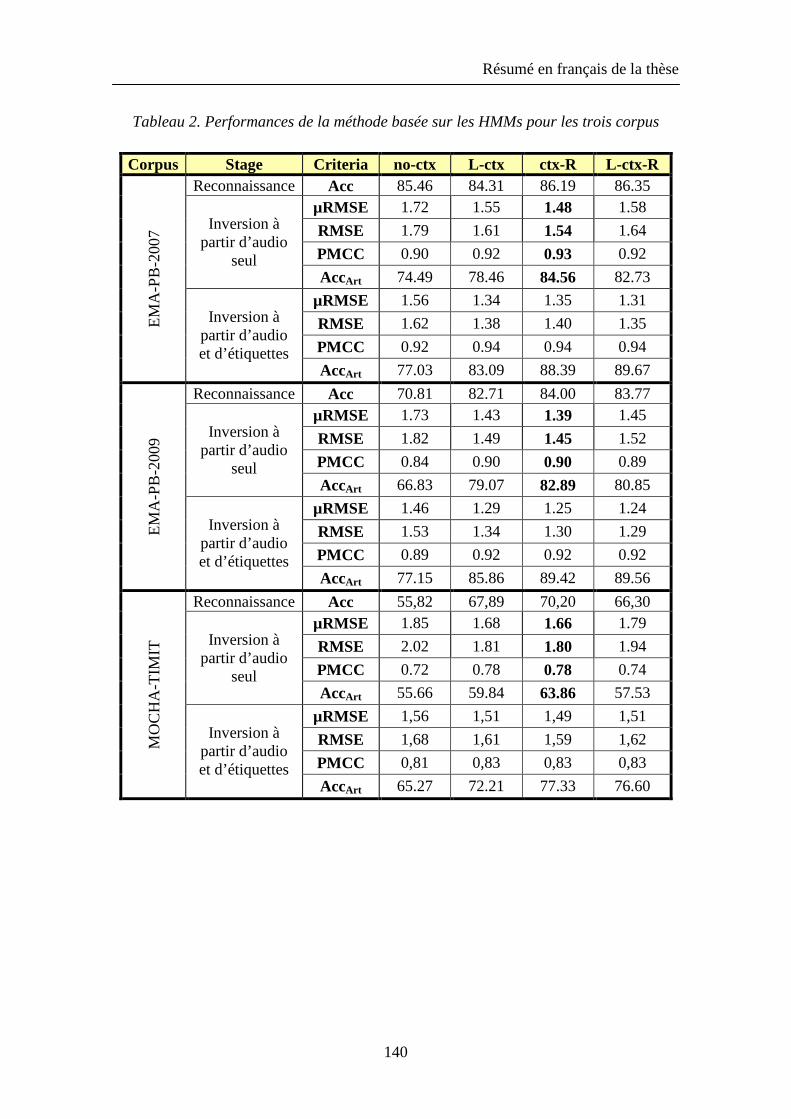
Résumé en français de la thèse
140
Tableau 2. Performances de la méthode basée sur les HMMs pour les trois corpus
Corpus Stage Criteria no-ctx L-ctx ctx-R L-ctx-R E
MA
-PB
-200
7
Reconnaissance Acc 85.46 84.31 86.19 86.35
Inversion à partir d’audio
seul
µRMSE 1.72 1.55 1.48 1.58
RMSE 1.79 1.61 1.54 1.64
PMCC 0.90 0.92 0.93 0.92
AccArt 74.49 78.46 84.56 82.73
Inversion à partir d’audio et d’étiquettes
µRMSE 1.56 1.34 1.35 1.31
RMSE 1.62 1.38 1.40 1.35
PMCC 0.92 0.94 0.94 0.94
AccArt 77.03 83.09 88.39 89.67
EM
A-P
B-2
009
Reconnaissance Acc 70.81 82.71 84.00 83.77
Inversion à partir d’audio
seul
µRMSE 1.73 1.43 1.39 1.45
RMSE 1.82 1.49 1.45 1.52
PMCC 0.84 0.90 0.90 0.89
AccArt 66.83 79.07 82.89 80.85
Inversion à partir d’audio et d’étiquettes
µRMSE 1.46 1.29 1.25 1.24
RMSE 1.53 1.34 1.30 1.29
PMCC 0.89 0.92 0.92 0.92
AccArt 77.15 85.86 89.42 89.56
MO
CH
A-T
IMIT
Reconnaissance Acc 55,82 67,89 70,20 66,30
Inversion à partir d’audio
seul
µRMSE 1.85 1.68 1.66 1.79
RMSE 2.02 1.81 1.80 1.94
PMCC 0.72 0.78 0.78 0.74
AccArt 55.66 59.84 63.86 57.53
Inversion à partir d’audio et d’étiquettes
µRMSE 1,56 1,51 1,49 1,51
RMSE 1,68 1,61 1,59 1,62
PMCC 0,81 0,83 0,83 0,83
AccArt 65.27 72.21 77.33 76.60
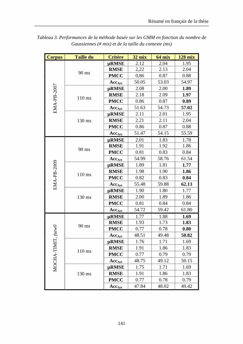
Résumé en français de la thèse
141
Tableau 3. Performances de la méthode basée sur les GMM en fonction du nombre de Gaussiennes (# mix) et de la taille du contexte (ms)
Corpus Taille du Critère 32 mix 64 mix 128 mix E
MA
-PB
-200
7
90 ms
µRMSE 2.12 2.04 1.95 RMSE 2,22 2.13 2.04 PMCC 0,86 0.87 0.88 AccArt 50.05 53.03 54.97
110 ms
µRMSE 2.08 2.00 1.89 RMSE 2.18 2.09 1.97 PMCC 0.86 0.87 0.89 AccArt 51.63 54.73 57.02
130 ms
µRMSE 2.11 2.01 1.95 RMSE 2.21 2.11 2.04 PMCC 0.86 0.87 0.88 AccArt 51.47 54.15 55.59
EM
A-P
B-2
009
90 ms
µRMSE 2.01 1.83 1.78 RMSE 1.91 1.92 1.86 PMCC 0.81 0.83 0.84 AccArt 54.99 58.76 61.54
110 ms
µRMSE 1.89 1.81 1.77 RMSE 1.98 1.90 1.86 PMCC 0.82 0.83 0.84 AccArt 55.48 59.88 62.13
130 ms
µRMSE 1.90 1.80 1.77 RMSE 2.00 1.89 1.86 PMCC 0.81 0.84 0.84 AccArt 54.72 59.42 61.80
MO
CH
A-T
IMIT
, fs
ew
0 90 ms
µRMSE 1.77 1.88 1.69 RMSE 1.93 1.73 1.83 PMCC 0.77 0.78 0.80 AccArt 48.51 49.48 50.82
110 ms
µRMSE 1.76 1.71 1.69 RMSE 1.91 1.86 1.83 PMCC 0.77 0.79 0.79 AccArt 48.75 49.12 50.15
130 ms
µRMSE 1.75 1.71 1.69 RMSE 1.91 1.86 1.83 PMCC 0.77 0.78 0.79
AccArt 47.84 48.02 49.42
Résumé en français de la thèse
142
5.2.2. Discussion
Nous avons analysé les résultats les meilleurs obtenus par les méthodes basées sur les HMMs et les GMMs en utilisant le corpus EMA-PB-2007. La RMSE globale obtenue pour l'inversion par HMMs (1,54 mm) est plus faible que celle obtenue par GMMs (1,96 mm). Un test de Student d’échantillons appariés a montré que la différence est significative (p <10-6). Ces résultats sont proches des résultats les plus élaborés de la littérature : Ling et al. (2010) ont trouvé 1,08 mm avec des HMMs alors que Zen et al. (2010) ont trouvé 1,13 mm avec des GMM de trajectoires. Une explication possible de des différences entre HMMs et GMMs pourrait être que les techniques basées sur les GMMs sont plus appropriées aux mises en correspondance unimodales où les événements dans la source et les cibles sont essentiellement synchrones, alors que des techniques basées sur les HMMs sont en mesure de traiter les deux flux différents et de pouvoir ainsi prendre en compte d’éventuelles asynchronies.
5.3. Relation entre mouvements faciaux et linguaux
Les techniques décrites ci-dessus pour l’inversion acoustique-articulatoire peuvent être appliquées d'une manière simple à la mise en correspondance lèvres / visage - langue. Depuis plus d'une décennie, la question de savoir si la forme la langue peut être prédite à partir de la forme des lèvres et du visage est toujours en débat ((Yehia et al., 1998), (Jiang et al., 2002), (Bailly and Badin, 2002), (Engwall and Beskow, 2003), (Beskow et al., 2003)). Ces études sont toutes basées sur une modélisation linéaire. Cette section présente ce problème avec les techniques de mise en correspondance plus sophistiquées que nous avons décrites ci-dessus, et compare les résultats avec ceux obtenus avec les modèles linéaires en utilisant les données articulatoires du corpus EMA-PB-2007. La forme des lèvres / visage a été représentée par les bobines de la mandibule et des lèvres, tandis que la langue était représentée par les trois autres bobines.
5.3.1. Prédiction de la langue par régression multilinéaire (MLR)
En utilisant la procédure validation croisée sur 5 partitions, l'inversion basée sur le modèle de régression linéaire multiple (Multi Linear Regression, MLR) a conduit à une RMSE de 3,88 mm et une PMCC de 0,59. Un expérience complémentaire sur un corpus réduit utilisant une répétition des VCVs, où C est l'une des 16 consonnes françaises et V = /i a u/ pour l’apprentissage, et l'autre répétition pour les tests, a conduit à une RMSE de 3,29 mm et un PMCC de 0,84, ce qui est comparable aux résultats des autres études. Lors de l'ajout de la voyelle /y/ - qui est connue pour être un sosie de la labiale /u/ en français – aux trois voyelles /i a u/, l’erreur RMSE s'élève à 3,67 mm et le PMCC diminue à 0,77, ce qui confirme la difficulté de prédire la forme la langue à partir de de celle des lèvres et du visage pour un certain nombre d'articulations.
Résumé en français de la thèse
143
5.3.2. Prédiction de la langue par HMMs
Nous avons obtenu les meilleurs résultats avec des modèles HMMs de phones en contexte gauche et droite avec une RMSE de 3,64 mm et un PMCC de 0,70.
Nous avons également constaté que l'utilisation des durées d’état produites par la reconnaissance faciale améliore de 4% environ l’erreur RMSE et le PMCC, par rapport à la méthode de z-score. Par ailleurs, nous avons également synthétisé les trajectoires de la langue directement à partir des étiquettes originales, en simulant une étape de reconnaissance faciale parfaite, afin d'évaluer la contribution de l’étape de synthèse à l’erreur d'inversion complète, comme nous l’avions fait pour l'inversion acoustico-articulatoire. On peut estimer que la contribution de la phase de synthèse de trajectoire à l’erreur RMSE globale est de 60% en moyenne; notons qu'elle était de près de 90% pour l’inversion acoustique-articulation décrite au-dessus. Cela montre que la reconnaissance faciale est beaucoup moins efficace que la reconnaissance acoustique.
5.3.3. Prédiction de la langue par GMMs
Nous avons constaté que l’erreur RMSE diminue lorsque le nombre de gaussiennes augmente. Pour 128 gaussiennes, et une taille de fenêtre de contexte optimale de 110 ms, nous avons trouvé une erreur RMSE de 2.90 mm et un PMCC de 0.80. L'interprétation la plus plausible est qu’une fenêtre de contexte de taille phonémique contient les indices phonétiques nécessaires pour l'inversion. En utilisant la phase supplémentaire de MLE, les résultats s’améliorent encore d’environ 5%.
5.3.4. Conclusion
Nous avons revisité le problème de la prédiction de la forme de la langue à partir de la forme des lèvres et du visage pour la parole. Nous avons évalué des méthodes de complexité différente et constaté que les GMMs donnent les résultats globaux meilleurs que les HMMs, tandis que la méthode MLR donne les résultats les plus mauvais. Les GMMs et les HMMs peuvent maintenir la répartition des classes phonétiques d'origine, avec quelques effets de centralisation ; ces effets de centralisation sont beaucoup plus forts avec la méthode MLR. Nous avons également montré que pour de grands corpus, la méthode MLR donne de mauvais résultats. Comme suggéré par Jiang et al. (2002), l’utilisation du contexte améliore assez bien les résultats. En conclusion, il n'est cependant pas possible de récupérer de manière fiable la forme de la langue à partir du visage dans le cas général.
6. Retour articulatoire multi-locuteur
Puisque notre objectif est de fournir un retour articulatoire visuel pour n’importe quel utilisateur, le système d'inversion doit être robuste et facile à adapter. Nous avons donc développé une phase d'adaptation acoustique qui permet à d’autres locuteurs d'utiliser le
Résumé en français de la thèse
144
système, bien que le retour articulatoire visuel soit limité à la tête parlante du locuteur de référence, et ne comporte pas les caractéristiques articulatoires spécifiques de l’utilisateur.
6.1. Inversion basée sur les HMMs
Pour l’étage d’adaptation de notre système, nous avons choisi la configuration suivante afin d’assurer les meilleurs résultats. Les modèles acoustiques et articulatoires HMMs initiaux ont été entraînés sur les quatre premières partitions du corpus EMA-PB-2007 pour des phones en contexte droit (ctx-R), puisqu’ils ont conduit aux meilleurs résultats d'inversion. Les HMMs acoustiques ont été entraînés en utilisant l'algorithme EM avec huit gaussiennes par état avec la technique d’états liés. Les HMMs articulatoires, représentés par une gaussienne par état, ont été entraînés en utilisant le critère MGE.
6.2. Adaptation acoustique du locuteur
Pour construire la base de données d'adaptation, l’utilisateur est invité à prononcer un ensemble de phrases qui sera utilisé comme corpus d'adaptation. La procédure d'adaptation est réalisée de la manière suivante. Tout d'abord, le signal de parole est automatiquement segmenté au niveau phonétique en utilisant un alignement forcé et les modèles acoustiques entrainés sur le sujet de référence. Ensuite, la technique de régression linéaire par maximum de vraisemblance (Maximum Likelihood Linear Regression, MLLR) est utilisée pour adapter chaque HMM acoustique. Cette étape supplémentaire rend les modèles de référence compatibles avec la voix de l’utilisateur, et permet aussi de prendre en compte un environnement acoustique différent. L'approche MLLR estime des transformations linéaires pour calculer les paramètres des modèles adaptés à partir des modèles initiaux afin de maximiser la probabilité des données d'adaptation (Leggetter and Woodland, 1995).
6.3. Expériences et résultats
6.3.1. Reconnaissance articulatoire
Puisque les données articulatoires ne sont pas disponibles pour les 3 locuteurs, il est impossible de déterminer la RMSE entre les trajectoires articulatoires mesurées et prédites. Par conséquent, nous avons réalisé l'évaluation de l’inversion pour ces locuteurs en appliquant une reconnaissance automatique articulatoire des 18 classes de phonème aux trajectoires inférées par inversion. La performance des modèles articulatoires entraînés sur les quatre premières partitions du corpus EMA-PB-2007 en utilisant des phones en contexte droit (ctx-R) est de 85,51 %. Ces HMMs articulatoires ont été ensuite utilisés pour évaluer les trajectoires articulatoires inversées pour tous les autres locuteurs.
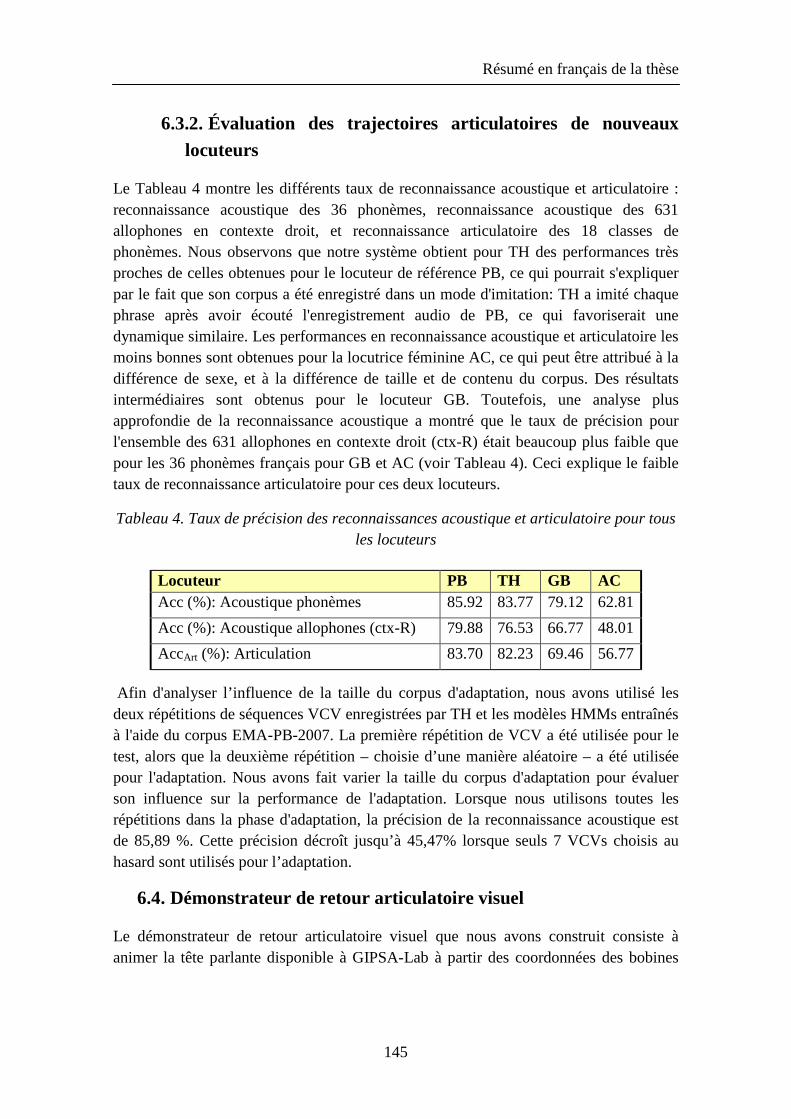
Résumé en français de la thèse
145
6.3.2. Évaluation des trajectoires articulatoires de nouveaux locuteurs
Le Tableau 4 montre les différents taux de reconnaissance acoustique et articulatoire : reconnaissance acoustique des 36 phonèmes, reconnaissance acoustique des 631 allophones en contexte droit, et reconnaissance articulatoire des 18 classes de phonèmes. Nous observons que notre système obtient pour TH des performances très proches de celles obtenues pour le locuteur de référence PB, ce qui pourrait s'expliquer par le fait que son corpus a été enregistré dans un mode d'imitation: TH a imité chaque phrase après avoir écouté l'enregistrement audio de PB, ce qui favoriserait une dynamique similaire. Les performances en reconnaissance acoustique et articulatoire les moins bonnes sont obtenues pour la locutrice féminine AC, ce qui peut être attribué à la différence de sexe, et à la différence de taille et de contenu du corpus. Des résultats intermédiaires sont obtenus pour le locuteur GB. Toutefois, une analyse plus approfondie de la reconnaissance acoustique a montré que le taux de précision pour l'ensemble des 631 allophones en contexte droit (ctx-R) était beaucoup plus faible que pour les 36 phonèmes français pour GB et AC (voir Tableau 4). Ceci explique le faible taux de reconnaissance articulatoire pour ces deux locuteurs.
Tableau 4. Taux de précision des reconnaissances acoustique et articulatoire pour tous les locuteurs
Locuteur PB TH GB AC Acc (%): Acoustique phonèmes 85.92 83.77 79.12 62.81
Acc (%): Acoustique allophones (ctx-R) 79.88 76.53 66.77 48.01
AccArt (%): Articulation 83.70 82.23 69.46 56.77
Afin d'analyser l’influence de la taille du corpus d'adaptation, nous avons utilisé les deux répétitions de séquences VCV enregistrées par TH et les modèles HMMs entraînés à l'aide du corpus EMA-PB-2007. La première répétition de VCV a été utilisée pour le test, alors que la deuxième répétition – choisie d’une manière aléatoire – a été utilisée pour l'adaptation. Nous avons fait varier la taille du corpus d'adaptation pour évaluer son influence sur la performance de l'adaptation. Lorsque nous utilisons toutes les répétitions dans la phase d'adaptation, la précision de la reconnaissance acoustique est de 85,89 %. Cette précision décroît jusqu’à 45,47% lorsque seuls 7 VCVs choisis au hasard sont utilisés pour l’adaptation.
6.4. Démonstrateur de retour articulatoire visuel
Le démonstrateur de retour articulatoire visuel que nous avons construit consiste à animer la tête parlante disponible à GIPSA-Lab à partir des coordonnées des bobines
Résumé en français de la thèse
146
EMA obtenues par inversion par la méthode utilisant les HMMs (voir Badin et al. (2010) pour le contrôle de la tête parlante à partir des coordonnées des bobines EMA).
Le démonstrateur de retour articulatoire visuel propose plusieurs options à l'utilisateur:
Enregistrement du signal audio pour les phrases proposées à l’utilisateur (VCV, CVC, phrases de corpus EMA-PB-2007). Le nombre de phrases à enregistrer est choisi par l'utilisateur.
Animation en ligne de la tête parlante à partir de la voix de l'utilisateur. Dans ce cas, les trajectoires articulatoires des bobines obtenues par inversion du signal audio de l'utilisateur sont utilisées pour animer la tête parlante. La séquence de phones reconnus est affichée pour donner une idée de la robustesse de la phase d'adaptation. Si la reconnaissance acoustique est mauvaise, l'enregistrement de phrases supplémentaires pour l’adaptation améliorera à la fois le résultat de la reconnaissance et l'inversion.
Animation hors ligne de la tête parlante à partir de fichiers de son et de trajectoires de bobines EMA associées.
7. Conclusions and perspectives
Nous avons développé un système de retour articulatoire visuel par inversion acoustico-articulatoire dans lequel les mouvements articulatoires reconstruits sont utilisés pour piloter une tête parlante virtuelle 3D. A notre connaissance, ce système n’a pas d’équivalent dans la littérature.
Dans ce but, nous avons mis en œuvre, évalué et comparé deux techniques d’inversion acoustico-articulatoire en parole qui diffèrent par la façon dont elles capturent et exploitent la cohérence multimodale a priori entre son et articulation. Ce travail se base sur des données acoustiques et articulatoires parallèles synchrones enregistrées à l’aide d’un articulographe électromagnétique.
Plusieurs remarques peuvent cependant être faites à propos de ces premières expériences. Les deux systèmes peuvent être améliorés. L’inversion à base de HMMs pourrait inclure un traitement plus sophistiqué de l’asynchronie articulatoire / acoustique en introduisant des modèles de retard qui se sont révélés efficaces pour la synthèse multimodale par HMMs (Govokhina et al., 2007). Le système basé sur les GMMs pourrait être amélioré en considérant d’autres techniques de réduction de la dimensionnalité telles que l’Analyse Discriminante Linéaire (LDA) qui sont assez efficaces pour l’inversion basée sur les HMMs (Tran et al., 2008). Les deux systèmes pourraient aussi gagner à incorporer de l’information visuelle en entrée et à inclure de manière plus intime cette information additionnelle dans le processus d’optimisation qui va considérer la cohérence multimodale entre les paramètres d’entrée et de sortie: en effet, les lèvres sont clairement visibles, et la position de la mâchoire est également accessible de manière indirecte à partir des mouvements faciaux.
Résumé en français de la thèse
147
Le traitement en temps réel constitue un élément important pour les travaux futurs. Il serait ainsi intéressant de mettre en œuvre l’algorithme de Viterbi à court terme proposé par Bloit and Rodet (2008) pour une implémentation temps réel des HMMs.
Un tel système de retour articulatoire visuel pourrait être intégré comme tuteur dans un système pour la correction phonétique (e.g. (Engwall and Bälter, 2007) ou (Badin et al., 2008a)). Badin et al. (2010) ont monté que les sujets ont des performances très diverses en lecture linguale, et que cette performance augmente avec l’entraînement. Notons ainsi que le réalisme du mouvement pourrait compenser le manque de précision des détails de forme: la cinématique des trajectoires calculées pourrait être plus importante pour la perception que la précision des trajectoires elles-mêmes.
8. Bibliographie
Atal, B. S., Chang, J. J., Mathews, M. V., and Tukey, J. W. (1978). "Inversion of articulatory-to-acoustic transformation in the vocal tract by a computer-sorting technique," Journal of the Acoustical Society of America 63, 1535-1555.
Badin, P., Elisei, F., Bailly, G., and Tarabalka, Y. (2008). "An audiovisual talking head for augmented speech generation: models and animations based on a real speaker's articulatory data," in Vth Conference on Articulated Motion and Deformable Objects (AMDO 2008, LNCS 5098), edited by F. J. Perales, and R. B. Fisher (Springer Verlag, Berlin, Heidelberg, Germany), pp. 132–143.
Badin, P., Tarabalka, Y., Elisei, F., and Bailly, G. (2010). "Can you 'read' tongue movements? Evaluation of the contribution of tongue display to speech understanding," Speech Communication 52, 493-503.
Bailly, G., and Badin, P. (2002). "Seeing tongue movements from outside," in 7th International Conference on Spoken Language Processing, ICSLP 2002 & Interspeech 2002 (Denver, Colorado, USA).
Ben Youssef, A., Badin, P., Bailly, G., and Heracleous, P. (2009). "Acoustic-to-articulatory inversion using speech recognition and trajectory formation based on phoneme hidden Markov models," in Proceedings of Interspeech 2009 (Brighton, UK), pp. 2255-2258.
Bernhardt, B. M., Bacsfalvi, P., Adler-Bock, M., Shimizu, R., Cheney, A., Giesbrecht, N., O'connell, M., Sirianni, J., and Radanov, B. (2008). "Ultrasound as visual feedback in speech habilitation: Exploring consultative use in rural British Columbia, Canada," Clinical Linguistics & Phonetics 22, 149-162.
Bernhardt, B. M., Gick, B., Bacsfalvi, P., and Adler-Bock, M. (2005). "Ultrasound in speech therapy with adolescents and adults," Clinical Linguistics & Phonetics 19, 605-617.
Résumé en français de la thèse
148
Bernhardt, B. M., Gick, B., Bacsfalvi, P., and Ashdown, J. (2003). "Speech habilitation of hard of hearing adolescents using electropalatography and ultrasound as evaluated by trained listeners," Clinical Linguistics & Phonetics 17, 199-216.
Beskow, J., Engwall, O., and Granström, B. (2003). "Resynthesis of facial and intraoral articulation from simultaneous measurements," in 15th International Congress of Phonetic Sciences, edited by M.-J. Solé, D. Recasens, and J. Romero (Barcelona, Spain), pp. 431-434.
Bloit, J., and Rodet, X. (2008). "Short-time Viterbi for online HMM decoding: Evaluation on a real-time phone recognition task," in Acoustics, Speech and Signal Processing, 2008. ICASSP 2008. IEEE International Conference on, pp. 2121-2124.
Chun, D. M. (2007). "Come ride the wave: But where is it taking us?," Calico Journal 24, 239-252.
Cucchiarini, C., Neri, A., and Strik, H. (2009). "Oral proficiency training in Dutch L2: The contribution of ASR-based corrective feedback," Speech Communication 51, 853-863.
Engwall, O., and Bälter, O. (2007). "Pronunciation feedback from real and virtual language teachers," Computer Assisted Language Learning 20, 235 - 262.
Engwall, O., and Beskow, J. (2003). "Resynthesis of 3D tongue movements from facial data," in Eurospeech 2003 (Geneva, Switzerland), pp. 2261-2264.
Fowler, C. A., Brown, J. M., Sabadini, L., and Weihing, J. (2003). "Rapid access to speech gestures in perception: Evidence from choice and simple response time tasks," Journal of Memory & Language 49, 396-413.
Govokhina, O., Bailly, G., and Breton, G. (2007). "Learning optimal audiovisual phasing for a HMM-based control model for facial animation," in 6th ISCA Workshop on Speech Synthesis (Bonn, Germany).
Hiroya, S., and Honda, M. (2004). "Estimation of articulatory movements from speech acoustics using an HMM-based speech production model," IEEE Trans. Speech and Audio Processing 12, 175-185.
Hueber, T., Chollet, G., Denby, B., and Stone, M. (2008). "Acquisition of ultrasound, video and acoustic speech data for a silent-speech interface application," in Proceedings of International Seminar on Speech Production (Strasbourg, France), pp. 365-369.
Jiang, J., Alwan, A. A., Keating, P. A., Auer, E. T., Jr, and Bernstein, J. (2002). "On the relationship between face movements, tongue movements, and speech acoustics," Special issue of EURASIP Journal on Applied Signal Provessing on joint audio-visual speech processing 2002, 1174-1188.
Résumé en français de la thèse
149
Kiritani, S. (1986). "X-Ray microbeam method for measurement of articulatory dynamics-techniques and results," Speech Communication 5, 119-140.
Leggetter, C., and Woodland, P. (1995). "Maximum likelihood linear regression for speaker adaptation of continuous density hidden Markov models," Computer, Speech and Language 9, 171-185.
Ling, Z.-H., Richmond, K., and Yamagishi, J. (2010). "An Analysis of HMM-based prediction of articulatory movements," Speech Communication 52, 834-846.
Menin-Sicard, A., and Sicard, E. (2006). "Evaluation et rééducation de la voix et de la parole avec Vocalab," Glossa 88, 62-76.
Neri, A., Cucchiarini, C., and Strik, H. (2002). "Feedback in computer assisted pronunciation training: technology push or demand pull?," in ICSLP-2002 (Denver, Co, USA), pp. 1209-1212.
Richmond, K. (2007). "Trajectory mixture density networks with multiple mixtures for acoustic-articulatory inversion," in Advances in Nonlinear Speech Processing (Lecture Notes in Computer Science 4885) (Springer Verlag, Berlin, Heidelberg, Germany), pp. 263-272.
Russell, G. O. (1928). "The vowel, its psychological mechanism, as shown by x-ray," in Columbus OH: Ohio State University Press.
Stone, M. (1990). "A three-dimensional model of tongue movement based on ultrasound and x-ray microbeam data," Journal of the Acoustical Society of America 87, 2207-2217.
Stone, M., Sonies, B., Shawker, T., Weiss, G., and Nadel, L. (1983). "Analysis of real-time ultrasound images of tongue configuration using a grid-digitizing system," Journal of Phonetics 11, 207–218.
Sumby, W. H., and Pollack, I. (1954). "Visual contribution to speech intelligibility in noise," Journal of the Acoustical Society of America 26, 212-215.
Toda, T., Black, A. W., and Tokuda, K. (2008). "Statistical mapping between articulatory movements and acoustic spectrum using a Gaussian mixture model," Speech Communication 50, 215-227.
Toutios, A., and Margaritis, K. (2005a). "Mapping the Speech Signal onto Electromagnetic Articulography Trajectories Using Support Vector Regression," in Text, Speech and Dialogue, edited by V. Matoušek, P. Mautner, and T. Pavelka (Springer, Berlin / Heidelberg), pp. 318-325.
Toutios, A., and Margaritis, K. (2005b). "A support vector approach to the acoustic-to-articulatory mapping," in Proceedings of Interspeech 2005 (Lisbon, Portugal), pp. 3221-3224.
Résumé en français de la thèse
150
Tran, V.-A., Bailly, G., Loevenbruck, H., and Jutten, C. (2008). "Improvement to a NAM captured whisper-to-speech system," in Interspeech (Brisbane, Australia), pp. 1465-1468.
Wrench, A., Gibbon, F., McNeill, A. M., and Wood, S. (2002). "An EPG therapy protocol for remediation and assessment of articulation disorders," in ICSLP-2002, pp. 965-968.
Wu, Y.-J., Wu, G., and Wang, R. H. (2006). "Minimum generation error criterion for tree-based clustering of context dependent HMMs," in Proceedings of Interspeech 2006 (Pittsburgh, USA), pp. 2046-2049.
Wu, Y. J., Zen, H., Nankaku, Y., and Tokuda, K. (2008). "Minimum generation error criterion considering global/local variance for HMM-based speech synthesis," in ICASSP (Las Vegas, NE, USA), pp. 4621-4624.
Yehia, H. C., Rubin, P. E., and Vatikiotis-Bateson, E. (1998). "Quantitative association of vocal-tract and facial behavior," Speech Communication 26, 23-43.
Young, S., Evermann, G., Gales, M., Hain, T., Kershaw, D., Liu, X. A., Moore, G., Odell, J., Ollason, D., Povey, D., Valtchev, V., and Woodland, P. (2009). "The HTK Book (for HTK Version 3.4). Revised for HTK Version 3.4 March 2009."
Zen, H., Nankaku, Y., and Tokuda, K. (2010). "Continuous Stochastic Feature Mapping Based on Trajectory HMMs," Audio, Speech, and Language Processing, IEEE Transactions on 19, 417-430.
Zen, H., Nankaku, Y., and Tokuda, K. (2011). "Continuous Stochastic Feature Mapping Based on Trajectory HMMs," Audio, Speech, and Language Processing, IEEE Transactions on 19, 417-430.
Zen, H., Tokuda, K., and Kitamura, T. (2004). "An introduction of trajectory model into HMM-based speech synthesis," in Fifth ISCA ITRW on Speech Synthesis (SSW5) (Pittsburgh, PA, USA), pp. 191-196.
Zhang, L. (2009). "Modelling Speech Dynamics with Trajectory-HMMs.," in The Centre for Speech Technology Research (School of Informatics, Edinburgh University, Edinburgh), p. 135.
Zhang, L., and Renals, S. (2008). "Acoustic-articulatory modeling with the trajectory HMM," IEEE Signal Processing Letters 15, 245-248.
Publications
151
Appendix B
Publications
Ben Youssef, A., Hueber, T., Badin, P. & Bailly, G. (2011). Toward a multi-speaker visual articulatory feedback system. In Interspeech 2011 (12th Annual Conference of the International Speech Communication Association). pp. 589-592. Florence, Italy, 28-31 August 2011.
Ben Youssef, A., Hueber, T., Badin, P., Bailly, G. & Elisei, F. (2011). Toward a speaker-independent visual articulatory feedback system. In 9th International Seminar on Speech Production, ISSP9. Montreal, Canada, 2011.
Ben Youssef, A., Badin, P. & Bailly, G. (2011). Improvement of HMM-based acoustic-to-articulatory speech inversion. In 9th International Seminar on Speech Production, ISSP9. Montreal, Canada, 2011.
Hueber, T., Badin, P., Bailly, G., Ben Youssef, A., Elisei, F., Denby, B. & Chollet, G. (2011). Statistical mapping between articulatory and acoustic data. Application to Silent Speech Interface and Visual Articulatory Feedback. In 1st International Workshop on Performative Speech and Singing Synthesis [P3S]. Vancouver, BC, Canada, 11-13 March 2011.
Badin, P., Ben Youssef, A., Bailly, G., Elisei, F. & Hueber, T. (2010). Visual articulatory feedback for phonetic correction in second language learning. In L2SW, Workshop on "Second Language Studies: Acquisition, Learning, Education and Technology", pp. P1-10. Tokyo, Japan, 22-24 September 2010.
Bailly, G., Badin, P., Revéret, L. & Ben Youssef, A. (in press). Sensori-motor characteristics of speech production. In Audiovisual speech (E. Vatikiotis-Bateson, G. Bailly & P. Perrier, editors), Cambridge, UK: Cambridge University Press.
Ben Youssef, A., Badin, P. & Bailly, G. (2010). Can tongue be recovered from face? The answer of data-driven statistical models. In Interspeech 2010 (11th Annual Conference of the International Speech Communication Association) (T. Kobayashi, K. Hirose & S. Nakamura, Eds.), pp. 2002-2005. Makuhari, Japan, 26-30 September 2010.
Ben Youssef, A., Badin, P. & Bailly, G. (2010). Acoustic-to-articulatory inversion in speech based on statistical models. In AVSP2010, 9th International Conference on Auditory-Visual Speech Processing (K. Sekiyama, S. Sakamoto, A. Tanaka, S. Tamura & C.T. Ishi, Eds.), pp. 160-165. Hakone, Kanagawa, Japan, September 30 - October 3 2010.
Ben Youssef, A., Tran, V.A., Badin, P. & Bailly, G. (2010). Méthodes basées sur les HMMs et les GMMs pour l’inversion acoustico-articulatoire en parole. In 28èmes Journées d'Etude de la Parole, pp. 249-252. Mons, Belgique, mai 2010.
Ben Youssef, A., Badin, P., Bailly, G. & Heracleous, P. (2009). Acoustic-to-articulatory inversion using speech recognition and trajectory formation based on phoneme hidden Markov models. In Interspeech 2009, pp. 2255-2258. Brighton, UK, 2009.
Ben Youssef, A., Tran, V.A., Badin, P. & Bailly, G. (2009). HMMs and GMMs based methods in acoustic-to-articulatory speech inversion. In VIIIèmes RJC Parole, pp. 186-192. Avignon, France, 16-18 novembre 2009.
Résumé
Cette thèse présente un système de retour articulatoire visuel, dans lequel les articulateurs visibles et non visibles d‘une tête parlante sont contrôlés par inversion à partir de la voix d'un locuteur. Notre approche de ce problème d‘inversion est basée sur des modèles statistiques élaborés à partir de données acoustiques et articulatoires enregistrées sur un locuteur français à l‘aide d‘un articulographe électromagnétique. Un premier système combine des techniques de reconnaissance acoustique de la parole et de synthèse articulatoire basées sur des modèles de Markov cachés (HMMs). Un deuxième système utilise des modèles de mélanges gaussiens (GMMs) pour estimer directement les trajectoires articulatoires à partir du signal acoustique. Pour généraliser le système mono-locuteur à un système multi-locuteur, nous avons implémenté une méthode d‘adaptation du locuteur basée sur la maximisation de la vraisemblance par régression linéaire (MLLR) que nous avons évaluée à l'aide un système de reconnaissance articulatoire de référence. Enfin, nous présentons un démonstrateur de retour articulatoire visuel.
Abstract
This thesis presents a visual articulatory feedback system in which the visible and non visible articulators of a talking head are controlled by inversion from a speaker’s voice. Our approach to this inversion problem is based on statistical models built on acoustic and articulatory data recorded on a French speaker by means of an electromagnetic articulograph. A first system combines acoustic speech recognition and articulatory speech synthesis techniques based on hidden Markov Models (HMMs). A second system uses Gaussian mixture models (GMMs) to estimate directly the articulatory trajectories from the speech sound. In order to generalise the single speaker system to a multi-speaker system, we have implemented a speaker adaptation method based on the maximum likelihood linear regression (MLLR) that we have assessed by means of a reference articulatory recognition system. Finally, we present a complete visual articulatory feedback demonstrator.