Progressive hedging-based metaheuristics for stochastic network design

Progressive Hedging-Based Metaheuristics forStochastic Network Design

Teodor Gabriel CrainicDépartement de management et technologie, École des sciences de la gestion, Université du Québec àMontréal, Montréal, CanadaInteruniversity Research Centre on Enterprise Networks, Logistics and Transportation (CIRRELT), Québec,Canada

Xiaorui FuDépartement d’informatique et de recherche opérationnelle, Université de Montréal, Montréal, CanadaInteruniversity Research Centre on Enterprise Networks, Logistics and Transportation (CIRRELT), Québec,Canada

Michel GendreauDépartement de mathématiques et de génie industriel, École Polytechnique de Montréal, Montréal, CanadaInteruniversity Research Centre on Enterprise Networks, Logistics and Transportation (CIRRELT), Québec,Canada

Walter ReiDépartement de management et technologie, École des sciences de la gestion, Université du Québec àMontréal, Montréal, CanadaInteruniversity Research Centre on Enterprise Networks, Logistics and Transportation (CIRRELT), Québec,Canada

Stein W. WallaceDepartment of Management Science, Management School, Lancaster University, Lancaster, United Kingdom

We consider the stochastic fixed-charge capacitated mul-ticommodity network design (S-CMND) problem withuncertain demand. We propose a two-stage stochasticprogramming formulation, where design decisions makeup the first stage, while recourse decisions are made inthe second stage to distribute the commodities accord-ing to observed demands. The overall objective is to

Received January 2009; accepted January 2011Correspondence to: T. G. Crainic; e-mail: [email protected] grant sponsor: Natural Sciences and Engineering Council of Canada(NSERC; Industrial Research Chairs and Discovery Grants programs), Part-ners of NSERC Industrial Research Chair, Canada Foundation for Innovation(Leaders Opportunity Fund, Ministère de l’éducation, du loisir et du sportdu Québec, SUN Microsystems, ILOG, and UQAM)Contract grant sponsor: The Research Council of Norway; Contract grantnumber: 171007/V30DOI 10.1002/net.20456Published online 2 August 2011 in Wiley Online Library(wileyonlinelibrary.com).© 2011 Wiley Periodicals, Inc.

optimize the cost of the first-stage design decisionsplus the total expected distribution cost incurred in thesecond stage. To solve this formulation, we proposea metaheuristic framework inspired by the progressivehedging algorithm of Rockafellar and Wets. Followingthis strategy, scenario decomposition is used to separatethe stochastic problem following the possible outcomes,scenarios, of the random event. Each scenario subprob-lem then becomes a deterministic CMND problem to besolved, which may be addressed by efficient specializedmethods. We also propose and compare different strate-gies to gradually guide scenario subproblems to agreeon the status of design arcs and aim for a good globaldesign. These strategies are embedded into a parallelsolution method, which is numerically shown to be com-putationally efficient and to yield high-quality solutionsunder various problem characteristics and demand cor-relations. © 2011 Wiley Periodicals, Inc. NETWORKS, Vol. 58(2),114–124 2011.

Keywords: stochastic network design; metaheuristics; progres-sive hedging; lagrangean relaxation

NETWORKS—2011—DOI 10.1002/net

1. INTRODUCTION

Fixed-charge capacitated multicommodity network design(CMND) models have been used to address many impor-tant planning problems in a variety of applications, such astransportation, logistics, and telecommunications [14,15]. Ingeneral terms, the CMND problem aims to design a networkthat is to be used to distribute a given set of commodi-ties between different pairs of origin and destination nodes.The design decisions consist in selecting the capacitatedarcs to include (open) in the network, a fixed cost havingto be paid whenever an arc is selected. The commoditiesare distributed through the resulting network to satisfy thedemand for transportation at minimum cost given, eventually,commodity-specific unit costs, while respecting the capacityof the selected arcs. The objective of the CMND problemconsists of finding a design that minimizes the total cost ofthe system computed as the sum of the total fixed cost andthe total distribution cost.

CMND problems were addressed in many settings (e.g.,transportation, Ref. [3]) through deterministic formulations,assuming that all necessary information was known at thetime design decisions were made and that these known val-ues were to be the same on repetitive utilizations of the design.This assumption is rarely observed in most realistic applica-tions; in general, uncertainty characterizes the future valuesof some or all parameters of interest. One such parameter,observed in almost all contexts, is the “demand” for trans-portation. The literature on stochastic CMND (S-CMND) isscarce, however. Our goal is to propose efficient metaheuris-tics for the S-CMND problem with uncertain demand.

In terms of decision and information process, the problemsetting that we address first determines a design based onsome estimation of the future commodity demand for trans-portation and, then, the resulting design serves repeatedly tooptimally flow a series of demand realizations using, even-tually, some external capacity. We formulate the problem asa two-stage stochastic programming formulation [1, 10], thedesign decisions making up the first stage, while recoursedecisions are made in the second stage to distribute theobserved commodity demands. Distribution costs are nowdependent on the latter and the objective becomes to finda design that minimizes the sum of the total fixed cost andthe total expected distribution cost (the recourse function).To address this model, we use the well-known approach ofapproximating the uncertain future through discretization ofthe probability distributions and the generation of a set ofscenarios, each scenario representing a possible realizationof the random event. The S-CMND problem thus becomes adeterministic mixed integer linear program of generally verylarge dimensions, which puts it beyond the capacity of exactsolution methods in all but trivial cases (the CMND problemsbelong to the NP-hard complexity class [14]).

We therefore propose a metaheuristic framework inspiredby the progressive hedging algorithm of Rockafellar and Wets[16] to address efficiently S-CMND problems with uncertaindemand. Convergence of the original progressive hedging

algorithm was proved for convex stochastic programs only,and it may not converge in the integer case. It provides, how-ever, the means to decompose the problem by scenarios andobserve that the differences between the respective designsmay be reflected as “penalties” to the fixed costs of the designarcs. This makes scenario subproblems addressable by effi-cient metaheuristics and provides ideas on how to use globallythe local information yielded by the subproblems, particu-larly when scenarios do not agree on arc status, to guide theoverall search mechanism toward a unique design vector.

The contribution of this article is twofold. First, wedevelop a metaheuristic framework, inspired by the progres-sive hedging strategy, which takes advantage of specializedmethods to solve deterministic CMND scenario subproblemsproblems. This type of approach was proposed [12] and suc-cessfully applied to the stochastic lot-sizing problem [6]. Toour knowledge, this article proposes the first such approachfor S-CMND problems with uncertain demand. Second, wepropose and compare different strategies aimed at gradu-ally guiding scenario subproblems to agree on the status ofdesign arcs and aim for a good (hopefully, optimal) globaldesign. These strategies are embedded into a parallel solutionmethod, which is numerically shown to be computationallyefficient and to yield high-quality solutions, under variousproblem characteristics and demand correlations.

The article is organized as follows. Section 2 presents theS-CMND formulation. The proposed metaheuristic isdescribed in Section 3. Section 4 is dedicated to the presenta-tion and analysis of the computational results. We concludein Section 5.

2. THE S-CMND FORMULATION

Let G = (N , A) be a network with node set N anddirected arc set A, and let K be the set of commodities,origin-destination pairs with non-negative demand, to be dis-tributed using this network. Define A = Aa ⋃ Ad, whereAa represents the set of “design arcs” among which theselection for the final network is to be made, while set Ad

includes a “dummy arc” for each commodity, that is, foreach pair of origin and destination nodes for which demandis defined. It is noteworthy that dummy arcs are generallynot included in standard deterministic CMND formulations[2, 14], but appear in many applications. In telecommu-nication, transportation, and logistics system planning, forexample, dummy arcs model the choice of using additionalresources from outside the system (e.g., outsourcing sometasks, renting capacity or equipment, etc.), or of delaying orrefusing service to all or part of the demand. In a stochas-tic setting, these actions are also part of recourse strategiesaddressing the part of realized demand exceeding the plannedcapacity of the network [11]. We include this option in therecourse strategy introduced later in this section. Define foreach design arc (i, j) ∈ Aa, the fixed cost fij incurred if thearc is included in the final design, and the capacity uij limit-ing the total commodity flow that may use it. Also define theunit transportation cost ck

ij for each commodity k ∈ K and arc

NETWORKS—2011—DOI 10.1002/net 115

(i, j) ∈ A, dummy arcs displaying much higher cost valuesthan those of design arcs.

Demand for deterministic CMND problems is expressedas vk units of commodity k ∈ K to be moved from its ori-gin o(k) ∈ N to its destination s(k) ∈ N . Several types ofuncertainty may be observed relative to this demand: volumesmay vary, some forecast demands might not materialize, or an“unexpected” demand might pop up for an origin-destinationnot previously considered. In this article, we focus on the firstcase, which is the most frequent and also includes the secondcase when appropriate value ranges are considered. Let therandom vector d define the demand distributions. Considerthe sample space � of random events that may be observedat the beginning of the second stage. For a given realizationω ∈ �, the demand distributions are fixed to d(ω), that is,for all i ∈ N and k ∈ K

dki (ω) =

vk(ω) if i = o(k),−vk(ω) if i = s(k),0 otherwise.

Define the design decision variables yij, (i, j) ∈ Aa, suchthat yij equals 1, when the design arc (i, j) is selected, and0, otherwise. The stochastic arc-based formulation of theCMND problem can then be written as:

min∑

(i,j)∈Aa

fijyij + Ed[Q(y, d(ω))] (1)

s.t. yij ∈ {0, 1}, ∀(i, j) ∈ Aa, (2)

where Q(y, d(ω)) equals the total distribution cost givendesign y, the realized demands d(ω), and a given recoursepolicy. The objective function (1) then minimizes the totalcost of the system as the sum of the total fixed costs incurredto build the system and the expected distribution costs asso-ciated with using it. Constraints (2) impose the integralityrequirements on the design variables.

Several recourse strategies could be considered, fromthe simple “observe and pay if not what planned for,” tocomplex procedures modifying the design and the flow dis-tribution over a number of stages. In this article, we considera single-stage, network recourse expressed as optimizingthe distribution of the observed demand using the networkdesigned in Stage 1 plus, when necessary, the extra capac-ity provided by the dummy arcs at a high (unit) price. Sucha strategy is appropriate when first-stage design decisionscannot be readily altered such as, for example, long-termmodifications to physical infrastructure or published sea-sonal transportation system schedules [11]. The second-stagerecourse function can then be formulated as a capacitatedmulticommodity minimum cost flow problem (CMMF)

Q(y, d(ω)) = min∑k∈K

∑(i,j)∈A

ckijx

kij (3)

s.t.∑

j∈N +(i)

xkij −

∑j∈N −(i)

xkji = dk

i (ω),

∀i ∈ N , ∀k ∈ K, (4)

∑k∈K

xkij ≤ uijyij, ∀(i, j) ∈ Aa, (5)

xkij ≥ 0, ∀(i, j) ∈ A, ∀k ∈ K, (6)

where decision variables xkij represents the flow of commodity

k ∈ K on arc (i, j) ∈ A, while N +(i) and N −(i) are thesets of outward and inward neighbors of node i, respectively.The objective function (3) minimizes the total distributioncost, Equations (4) enforce the flow conservation constraints(dummy arcs are considered), and relations (5) impose thecapacity restrictions on the design arcs of the network.

3. THE PROGRESSIVE HEDGING-BASEDMETAHEURISTIC

This section introduces the metaheuristic that we proposeto address efficiently stochastic CMND problems. Inspired bythe progressive hedging algorithm of Rockafellar and Wetts[16], one first applies a scenario decomposition technique toseparate the stochastic problem following the possible out-comes, or scenarios, of the random event (Section 3.1). Thisyields a series of scenario subproblems that take the formof CMND formulations with modified fixed costs, for whichefficient metaheuristics exist (e.g., Ref. [5]). The fixed costsof the scenario subproblems are modified to reflect the dif-ferences that may exist between the “local” scenario designsand an overall design extracted from these, which serves as areference point. A heuristic search procedure then iterativelycomputes an overall design as the expectation over the currentsolutions of the scenario subproblems (Section 3.2), adjuststhe modified fixed costs to aim for a “consensus” design(Section 3.3), and solves the scenario subproblems (Section3.4). The last phase of the metaheuristic solves a reduced mul-tiscenario formulation on the design arcs for which consensushas not been reached through the iterative search phase.

Rockafellar and Wetts [16] proposed the progressive hedg-ing algorithm based on an augmented Lagrangean strategythat converges to a global optimum in the case of continuousstochastic problems. They also remarked that this strategymay not converge in the integer case and, thus, the attemptsto apply this approach to integer programming formulations(e.g., Ref. [6,9,12]) resulted in heuristics. We follow the samestrategy and propose a metaheuristic.

It is important to notice that the metaheuristic does not aimto force consensus among scenarios at all costs. It is actuallyknown that, because subproblems are deterministic, even ifall scenarios agree on a certain aspect of the solution, forexample, including a specific arc in the overall design, thereis no guarantee that this will be part of the final solution [17].Only when the scenarios agree on all elements of the solution,thus producing the same design, can conclusions be drawn.This is particularly true in the first iterations of the algorithm,when very little exchanges have taken place among scenariosand the fixed cost adjustments are negligible. We are thuscareful not to apply any ideas of variable fixing based onscenario agreement until the metaheuristic has been run for

116 NETWORKS—2011—DOI 10.1002/net

quite a while and parameters have been adjusted. The goalis to gradually bring out the compromise solution among thediverse demand realizations of the sampled scenarios, playingon trade-offs between the cost of setting up a network and thatof calling on external capacity.

3.1. Scenario Decomposition for the Stochastic CMNDFormulation

Let S ⊆ � define a set of possible scenarios for the ran-dom event. One can then approximate the stochastic CMNDformulation through a multiscenario deterministic model

min∑

(i,j)∈Aa

fijyij +∑s∈S

ps

∑

k∈K

∑(i,j)∈A

ckijx

ksij

, (7)

s.t.∑

j∈N +(i)

xksij −

∑j∈N −(i)

xksji = dks

i

∀i ∈ N , ∀k ∈ K, ∀s ∈ S, (8)∑k∈K

xksij ≤ uijyij ∀(i, j) ∈ Aa, ∀s ∈ S, (9)

yij ∈ {0, 1} ∀(i, j) ∈ Aa, (10)

xksij ≥ 0 ∀(i, j) ∈ A, ∀k ∈ K, ∀s ∈ S, (11)

where ps defines the probability of scenario s ∈ S, whilethe commodity flow variables and the, now deterministic,demands are scenario specific. Model (7)–(11) is a large-scale mixed integer prgram with a block-diagonal structure,each block, defined by constraints (8) and (9), representinga CMMF problem for a scenario s ∈ S. By solving problem(7)–(11), one finds a single design yij that minimizes the sumof fixed costs and expected distribution costs over all thescenarios.

Constraints (9) link the first- and second-stage variablesand force the flow distribution to use only the capacity ofthe arcs selected in the first stage. Creating a copy ys

ij ∈{0, 1}, (i, j) ∈ Aa, of the first-stage variables for eachscenario s ∈ S yields the formulation

min∑s∈S

ps

∑

(i,j)∈Aa

fijysij +

∑k∈K

∑(i,j)∈A

ckijx

ksij

(12)

s.t.∑k∈K

xksij ≤ uijy

sij ∀(i, j) ∈ Aa, ∀s ∈ S, (13)

ysij = yt

ij ∀s, t ∈ S, s �= t, (14)

ysij ∈ {0, 1} ∀(i, j) ∈ Aa, ∀s ∈ S, (15)

plus constraints (8) and (11), which is scenario-separablethrough the relaxation of the “nonanticipativity constraints”(14). The latter make sure design decisions are not tai-lored for each particular scenario and aim to yield a “singleimplementable design” [16].

The number of constraints (14) may be quite large,however, and they are therefore replaced with

ysij = yij ∀(i, j) ∈ Aa, ∀s ∈ S, (16)

yij ∈ {0, 1} ∀(i, j) ∈ Aa, (17)

where yij ∈ {0, 1}, (i, j) ∈ Aa, is defined as the “overalldesign vector.” Then, following the decomposition schemeproposed in Rockafellar and Wets [16], constraints (16)are relaxed using an augmented Lagrangean strategy, whichyields the objective function

min∑s∈S

ps

∑

(i,j)∈Aa

fijysij +

∑k∈K

∑(i,j)∈A

ckijx

ksij

+∑

(i,j)∈Aa

λsij(y

sij − yij) + 1

2

∑(i,j)∈Aa

ρ(ysij − yij)

2

, (18)

with Lagrangean multipliers λsij, (i, j) ∈ Aa, s ∈ S, for the

relaxed constraints, and a penalty ratio ρ. Given the binaryrequirements for the design variables, the function may bereduced to

min∑s∈S

ps

∑

(i,j)∈Aa

(fij + λs

ij − ρyij + ρ

2

)ys

ij

+∑

(i,j)∈A

∑k∈K

ckijx

ksij

−

∑(i,j)∈Aa

λsijyij +

∑(i,j)∈Aa

1

2ρyij. (19)

For a given overall design yij, the relaxed formulation thendecomposes by scenario, each scenario subproblem s takingthe form of a deterministic CMND problem with modifiedfixed costs

min∑

(i,j)∈Aa

(fij + λs

ij − ρyij + ρ

2

)ys

ij +∑

(i,j)∈A

∑k∈K

ckijx

ksij

(20)

s.t.∑

j∈N +(i)

xksij −

∑j∈N −(i)

xksji = dks

i ∀i ∈ N , ∀k ∈ K,

(21)∑k∈K

xksij ≤ uijy

sij ∀(i, j) ∈ Aa, (22)

ysij ∈ {0, 1} ∀(i, j) ∈ Aa, (23)

xksij ≥ 0 ∀(i, j) ∈ A, ∀k ∈ K, (24)

which may be addressed by a variety of exact and meta-heuristic solution methods (see, e.g., the survey of Crainicand Kim [3]).

For a given scenario subproblem s, the Lagrangean mul-tiplier λs

ij and the parameter ρ contribute to penalize thedifference in terms of the values of the design arcs between


the local design and the current overall design. We now exam-ine the proposed strategies to, first, extract the overall designand, second, adjust the fixed costs of the scenario subproblemdesign variables to guide the search toward consensus amongthe scenario designs.

3.2. Extracting an Overall Design

The goal of this step of the metaheuristic is to take advan-tage of the local information provided by the scenario designsto produce an overall design to serve as reference point forall scenarios. Let ν define the iteration index of the meta-heuristic sketched at the beginning of this section. We needto define an aggregation operator in order to combine thescenario designs into a single design given a weight for eachscenario s ∈ S. In Ref. [16], the average function given thescenario probabilities was used as the aggregation operator.When transposed to the present problem, this yields

yνij =

∑s∈S

psysνij , ∀(i, j) ∈ Aa. (25)

When all scenarios agree on the selection status for anarc (i, j) ∈ Aa, one obtains yν

ij ∈ {0, 1}. Then, if consensusis observed for all design arcs, the optimal design has beenobtained and the procedure stops. Most of the time this isnot the case, however, and one observes 0 < yν

ij < 1 for anumber of design arcs, which is infeasible given the integral-ity requirements of the design variables. Therefore, operator(25) does not necessarily produce an overall feasible design.Moreover, as recalled at the beginning of the section, one can-not even expect that a good solution will be obtained. Yet, thisoperator may still be used to identify trends among scenariosolutions and guide this phase of the metaheuristic. Thus,for a nonconsensus arc (i, j), a low, close to zero, value foryν

ij indicates a trend toward closing the arc. Symmetrically, avalue close to one indicates a trend to open the arc. We there-fore use (25) to produce a reference point within the searchphase of the metaheuristic with the objective of identifying asubset of arcs for which consensus appears possible.

Note that, a worst-case analysis always yields a solution,denoted “max design,”

yMνij =

∨s∈S

ysνij , ∀(i, j) ∈ Aa, (26)

where an arc is open as soon as at least one scenario selectsit. The max design solution is feasible for problem (7)–(11)and

∑(i,j)∈Aa fijyMν

ij + ∑s∈S psQ(yMν , ds) yields an upper

bound on its optimal value. Solutions given by (26) are notappropriate as reference points, however, because max designmay create a bias in the search process toward producingunnecessarily large overall designs. We compute it iterativelyduring the search phase, however, to keep a best upper bound.

3.3. Metaheuristic Search for a Good Global Design

We present two strategies to dynamically adjust the fixedcosts of the CMND scenario subproblems to gradually aim

for a consensus on the arcs to include or not in the overalldesign. The first, described in section 3.3.1, adjusts the fixedcosts indirectly by working with the augmented Lagrangeanparameters, whereas the second, in section 3.3.2, adjusts thefixed costs directly.

3.3.1. Modifying the Lagrangean Parameters. The firststrategy is inspired by the augmented Lagrangean method(see, for instance, Ref. [13] for a general description) andmodifies the Lagrangean multipliers and the ρ parameterassociated to the non-anticipativity constraints (the strategyused in Ref. [12] proceeds from similar ideas). As alreadyindicated, because of the integrality of the decision variables,the “local” convexity and global convergence properties ofthe augmented Lagrangean method do not apply in this case.The proposed strategy is thus a heuristic, where the multi-plier modifications aim to give an incentive to open or closean arc when its status is different from that in the current ref-erence point, the incentive being gradually strengthened asthe penalty factor is slowly increased.

Let λsνij be the value of the Lagrangean multiplier asso-

ciated with the nonanticipativity constraint for the designdecision on arc (i, j) for scenario s, at iteration ν, and ρν

be the value of the quadratic penalty at the same iteration.The parameters are then updated as follows:

λsνij ← λsν−1

ij + ρν−1(ysνij − yν−1

ij

), ∀(i, j) ∈ Aa, (27)

ρν ← αρν−1, (28)

where the initial value ρ0 is set to a small positive value, aswell as the constant α > 1, which makes for a slow increasein the penalty term.

The idea follows the observation that there are threepossible adjustments for any design arc (i, j) in a scenariosubproblem s, at iteration ν:

1. ysνij < yν−1

ij . In this case, the arc is closed in the scenario

design but not in the reference point (0 < yν−1ij < 1).

The idea is then to reduce the fixed cost of the arc in thescenario subproblem to give an incentive to open it.

2. ysνij > yν−1

ij . The symmetric case where the arc is openedin the scenario design, but not all other scenarios agree.The fixed cost is adjusted so as to give an incentive toclose the arc within the scenario design. Notice that thisadjustment is stronger when most of the other scenariosclosed the arc (low value of yν−1

ij ).

3. ysνij = yν−1

ij and there is consensus amongst the scenariodesigns regarding the status of the arc and the fixed costremains unchanged.

It is important to note that if the value chosen for ρ0 istoo large, the procedure will converge prematurely and, mostprobably, to a design that may be quite far from an optimalone. However, this situation may be easily detected by notingthat in such a case the method will perform just a few itera-tions. Should this occur, the algorithm should be restartedwith a much smaller value of ρ0. In our computationalexperiments, we did not encounter such situations.


3.3.2. Heuristic Strategy. We introduce a new heuristicadjustment strategy that at each iteration modifies the fixedcosts of the design arcs with a status different from what amajority of the other arcs agree upon at the current iteration.The objective is, as before, to incite the scenario subproblemsto agree on a design optimal for all. Two adjustments areproposed, one at the level of the reference point and the otherwithin each scenario.

Starting from the reference point yνij at iteration ν, the

global adjustment attempts to favor what appears as the cur-rent trend amongst the scenario designs to open or close arc(i, j). A low value of yν

ij indicates that arc (i, j) is opened onlyin a small number of scenario designs, while a high valuemeans that arc (i, j) is opened within a majority of scenariodesigns. One can then argue that when yν

ij is less than a given

threshold clow, increasing the fixed cost of arc (i, j) may drivethe subproblems to avoid using it. On the other hand, whenyν

ij is higher than a given threshold chigh, lowering the fixedcost of arc (i, j) should attract the scenario subproblems touse it. In the current implementation, “low” and “high” aredefined as less and more than half the scenarios, respectively.The global adjustment strategy is then defined as

f νij =

βf ν−1ij if yν−1

ij < clow,

1

βf ν−1ij if yν−1

ij > chigh,

f ν−1ij otherwise,

(29)

with parameters β > 1, 0 < clow < 0.5, and 0.5 < chigh < 1,and f ν

ij representing the modified fixed cost of arc (i, j) in allscenarios.

A second adjustment is performed at the level of each sce-nario s ∈ S for which there are arcs with “large” differencesbetween the values of the local design ysν

ij and the currentreference point yν

ij:

f sνij =

βf νij if

∣∣ysν−1ij − yν−1

ij

∣∣ ≥ cfar and ysν−1ij = 1,

1

βf νij if

∣∣ysν−1ij − yν−1

ij

∣∣ ≥ cfar and ysν−1ij = 0,

f νij otherwise,

(30)

with parameters β > 1, 0.5 < cfar < 1 representing thethreshold defining when a local adjustment is to be applied,and f sν

ij standing for the modified local fixed cost of arc (i, j)for scenario s at iteration ν.

One can exploit this idea a bit further by examining thearcs that in the design of scenario s appear close to the currentreference point, that is, those for which |ysν−1

ij −yν−1ij | ≤ cnear,

for a consensus threshold 0 < cnear < 0.5. One may thendecide that, locally, one does not desire to modify the statusof these arcs and fix them for the next iteration by settingysν

ij = ysν−1ij , thus yielding a smaller CMND problem that

may be solved more rapidly.

3.4. The Complete Metaheuristic

Algorithm 1 sums up the entire procedure, where theLagrangean-based and heuristic fixed cost adjustment strate-gies are identified as (L) and (H), respectively. In the currentimplementation, the initial scenario subproblem solutionsare simply obtained by opening all arcs, solving the relatedCMMF problem, and closing the unused arcs. Later, at eachiteration of the global metaheuristic, each subproblem issolved starting from the solution at the previous iteration.

For each scenario and iteration, the resulting subproblemis a deterministic CMND with possibly modified fixed costs.To address these problems, we use one of the currently bestprocedures for the CMND, the cycle-based tabu search ofGhamlouche et al. [5], which explores the space of the arc-design variables by redirecting flow around cycles and closingand opening design arcs accordingly.

Algorithm 1 The S-CMND metaheuristic with fixed-costadjustment L or H

Initialization• ν ← 0;• If L = true, then λsν

ij ← 0, ∀(i, j) ∈ Aa, ∀s ∈ S; ρν ←ρ0;

• for all s ∈ S dof sνij ← fij , ∀(i, j) ∈ Aa;

Solve the corresponding CMND subproblem;• yν

ij ← ∑s∈S psysν

ij , ∀(i, j) ∈ A;

• BestSolution ← yMν ;

while stopping criterion not met do• ν ← ν + 1;• If H = true, then, adjust globally f ν

ij , ∀(i, j) ∈ Aa usingEquation (29);

• for all s ∈ S doIf L = true, then, f sν

ij ← fij +λsν−1ij −ρν−1yν−1

ij + ρν−1

2 ,∀(i, j) ∈ Aa;

If H = true, then, adjust locally f sνij , ∀(i, j) ∈ Aa using

Equation (30);Fix some ysν

ij as appropriate;

Solve the corresponding CMND subproblem;• Update

yνij ← ∑

s∈S psysνij

If L = true, then, λsνij ← λsν−1

ij + ρν−1(ysνij −

yν−1ij )∀(i, j) ∈ Aa;

ρν ← αρν−1;

Update bestSolution = yMν when appropriate;

Second Phase• Fix the design variables for which consensus is obtained;• Solve the restricted multi-scenario CMND formulation.

As indicated earlier on, there are no theoretical criteriafor the convergence of the progressive hedging-based algo-rithms in the integer case. To obtain a unique design, wetherefore proceed in two phases. We proceed with the search


as described previously and stop it either when consensus isobtained on all design arcs, or when the first of several classi-cal metaheuristic criteria is satisfied, namely, reaching a totalof 50 iterations, 10 consecutive nonimproving iterations, or10 h of CPU time. The second phase then solves the restrictedstochastic CMND obtained by fixing all design arcs for whichconsensus has been achieved.

4. EXPERIMENTATION

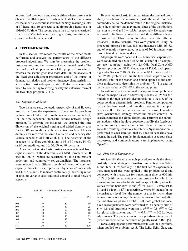
In this section, we report the results of the experimentsperformed and analyze the performance of the differentproposed algorithms. We start by presenting the probleminstances used, and then two sets of experimental results. Thefirst makes a first appreciation of the proposed procedures,whereas the second goes into more detail in the analysis ofthe fixed-cost adjustment procedures and of the impact ofdemand correlation and problem-instance characteristics interms of fixed cost and capacity ratios. Performances are eval-uated by comparing to solving exactly the extensive form ofthe two-stage program (7–11).

4.1. Experimental Setup

Two instance sets, denoted, respectively, S and R, wereused to perform the experiments. There are 16 problemsincluded in set S derived from the instances used in Ref. [7]for the time-dependent stochastic service network designproblem. To generate the instances, we dropped the timedimension of the original setting and added dummy arcsfor the OD commodities of the respective problem. All non-dummy arcs received the same fixed-cost and capacity (thevehicle capacities of Hoff et al. [7]). The networks of theinstances in set S are combinations of 16 or 30 nodes, 14, 40,or 80 commodities, and 10, 20, 60, or 90 scenarios.

A second set of stochastic instances was obtained fromeight instances of the deterministic CMND problem set Rused in Ref. [5], which are described in Table 1 in terms ofnode, arc, and commodity set cardinalities. The instanceswere selected with different combined levels of cost andcapacity characteristics, represented by a “ratio” index val-ued 1, 3, 5, 7, and 9 to indicate continuously increasing ratiosof fixed to variable costs and total demand to total networkcapacity.

TABLE 1. Attributes of R instances.

Name |N | |A| |K|

r04 10 60 10r05 10 60 25r06 10 60 50r07 10 82 10r08 10 83 25r09 10 83 50r10 20 120 40r11 20 120 100

To generate stochastic instances, triangular demand prob-ability distributions were assumed, with the mode c of eachcommodity set to the demand value in the original instance,while the minimum and maximum values of the distributionswere set to a = 0 and b = 1.35c, respectively. Demands wereassumed to be linearly correlated and three different levelsof positive correlations were considered to create differentinstances. Finally, scenario trees were generated using theprocedure proposed in Ref. [8], and instances with 16, 32,and 64 scenarios were created. A total of 360 instances werethus obtained in this second set.

All programs were coded in C++. Numerical experimentswere conducted on a Sun Fire X4100 cluster of 16 comput-ers, each computer having two 2.6-GHz Dual-Core AMDOpteron processors. 8192 Megabytes of RAM, and operat-ing under Solaris 2.10. cplex version 10.1.1 was used forthe CMMF problems within the tabu search applied to eachscenario, and for the branch-and-bound applied to the com-plete multiscenario deterministic problem (7)–(11) and therestricted stochastic CMND in the second phase.

As with most other combinatorial optimization problems,one of the major issues in addressing stochastic CMND for-mulations through scenario decomposition is the size of thecorresponding deterministic problem. Parallel computationcan and has been used to address this issue and it is adoptedhere as well. In the current version, we use a simple master-slave synchronous strategy, where the master controls thesearch, computes the global design, and performs the param-eter updates, while the slave processors modify the fixed costsaccording to the information received from the master andsolve the resulting scenario subproblems. Synchronization isperformed at each iteration, that is, once all scenarios havebeen addressed. The parallel implementation used four slaveprocessors, and communications were implemented usingOpenMP.

4.2. First Set of Experiments

We identify the tabu search procedures with the fixed-cost adjustment strategies formalized in Section 3 as Tabu-L and Tabu-H, respectively. In the first set of experiments,these metaheuristics were applied to the problem set S andcompared with cplex run for a maximum time of 600 minof CPU (with the exception of one instance for which themaximum time was doubled). With respect to the parametervalues for the heuristics, α and ρ0 for TABU-L were set to1.1 and 1+ log(1+D0), respectively, where D0 stands for theinconsistency level (i.e., the number of arcs for which thereis nonconsensus amongst the initial scenario solutions) afterthe initialization phase. For TABU-H, both global and localfixed cost adjustments were performed with a penalty ratio ofβ = 1.1, and thresholds were set to chigh = 0.8, clow = 0.2for global adjustments, and cfar = 0.7, cnear = 0.2 for localadjustments. The parameters of the cycle-based tabu searchprocedure were set to the values originally used in Ref. [5].

Table 2 displays the performance results of the algorithmswhen applied to problem set S. The L.B., U.B., Gap, and


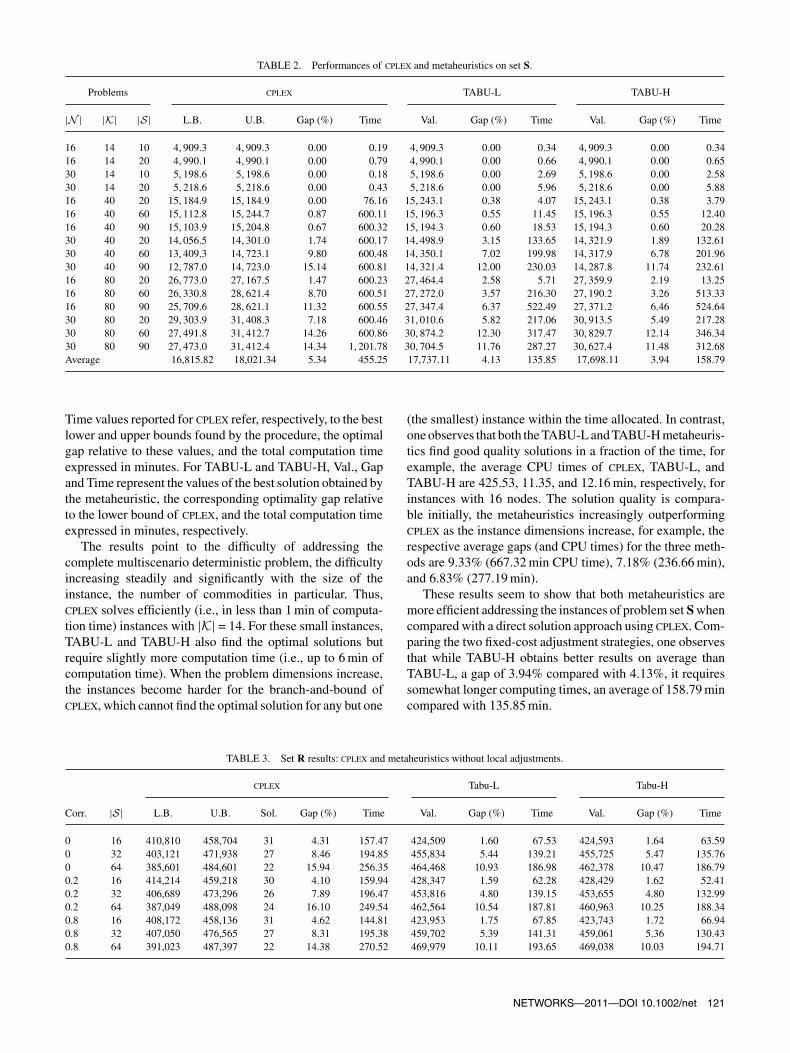
TABLE 2. Performances of cplex and metaheuristics on set S.

Problems cplex TABU-L TABU-H

|N | |K| |S| L.B. U.B. Gap (%) Time Val. Gap (%) Time Val. Gap (%) Time

16 14 10 4, 909.3 4, 909.3 0.00 0.19 4, 909.3 0.00 0.34 4, 909.3 0.00 0.3416 14 20 4, 990.1 4, 990.1 0.00 0.79 4, 990.1 0.00 0.66 4, 990.1 0.00 0.6530 14 10 5, 198.6 5, 198.6 0.00 0.18 5, 198.6 0.00 2.69 5, 198.6 0.00 2.5830 14 20 5, 218.6 5, 218.6 0.00 0.43 5, 218.6 0.00 5.96 5, 218.6 0.00 5.8816 40 20 15, 184.9 15, 184.9 0.00 76.16 15, 243.1 0.38 4.07 15, 243.1 0.38 3.7916 40 60 15, 112.8 15, 244.7 0.87 600.11 15, 196.3 0.55 11.45 15, 196.3 0.55 12.4016 40 90 15, 103.9 15, 204.8 0.67 600.32 15, 194.3 0.60 18.53 15, 194.3 0.60 20.2830 40 20 14, 056.5 14, 301.0 1.74 600.17 14, 498.9 3.15 133.65 14, 321.9 1.89 132.6130 40 60 13, 409.3 14, 723.1 9.80 600.48 14, 350.1 7.02 199.98 14, 317.9 6.78 201.9630 40 90 12, 787.0 14, 723.0 15.14 600.81 14, 321.4 12.00 230.03 14, 287.8 11.74 232.6116 80 20 26, 773.0 27, 167.5 1.47 600.23 27, 464.4 2.58 5.71 27, 359.9 2.19 13.2516 80 60 26, 330.8 28, 621.4 8.70 600.51 27, 272.0 3.57 216.30 27, 190.2 3.26 513.3316 80 90 25, 709.6 28, 621.1 11.32 600.55 27, 347.4 6.37 522.49 27, 371.2 6.46 524.6430 80 20 29, 303.9 31, 408.3 7.18 600.46 31, 010.6 5.82 217.06 30, 913.5 5.49 217.2830 80 60 27, 491.8 31, 412.7 14.26 600.86 30, 874.2 12.30 317.47 30, 829.7 12.14 346.3430 80 90 27, 473.0 31, 412.4 14.34 1, 201.78 30, 704.5 11.76 287.27 30, 627.4 11.48 312.68Average 16,815.82 18,021.34 5.34 455.25 17,737.11 4.13 135.85 17,698.11 3.94 158.79

Time values reported for cplex refer, respectively, to the bestlower and upper bounds found by the procedure, the optimalgap relative to these values, and the total computation timeexpressed in minutes. For TABU-L and TABU-H, Val., Gapand Time represent the values of the best solution obtained bythe metaheuristic, the corresponding optimality gap relativeto the lower bound of cplex, and the total computation timeexpressed in minutes, respectively.

The results point to the difficulty of addressing thecomplete multiscenario deterministic problem, the difficultyincreasing steadily and significantly with the size of theinstance, the number of commodities in particular. Thus,cplex solves efficiently (i.e., in less than 1 min of computa-tion time) instances with |K| = 14. For these small instances,TABU-L and TABU-H also find the optimal solutions butrequire slightly more computation time (i.e., up to 6 min ofcomputation time). When the problem dimensions increase,the instances become harder for the branch-and-bound ofcplex, which cannot find the optimal solution for any but one

(the smallest) instance within the time allocated. In contrast,one observes that both the TABU-L and TABU-H metaheuris-tics find good quality solutions in a fraction of the time, forexample, the average CPU times of cplex, TABU-L, andTABU-H are 425.53, 11.35, and 12.16 min, respectively, forinstances with 16 nodes. The solution quality is compara-ble initially, the metaheuristics increasingly outperformingcplex as the instance dimensions increase, for example, therespective average gaps (and CPU times) for the three meth-ods are 9.33% (667.32 min CPU time), 7.18% (236.66 min),and 6.83% (277.19 min).

These results seem to show that both metaheuristics aremore efficient addressing the instances of problem set S whencompared with a direct solution approach using cplex. Com-paring the two fixed-cost adjustment strategies, one observesthat while TABU-H obtains better results on average thanTABU-L, a gap of 3.94% compared with 4.13%, it requiressomewhat longer computing times, an average of 158.79 mincompared with 135.85 min.

TABLE 3. Set R results: cplex and metaheuristics without local adjustments.

cplex Tabu-L Tabu-H

Corr. |S| L.B. U.B. Sol. Gap (%) Time Val. Gap (%) Time Val. Gap (%) Time

0 16 410,810 458,704 31 4.31 157.47 424,509 1.60 67.53 424,593 1.64 63.590 32 403,121 471,938 27 8.46 194.85 455,834 5.44 139.21 455,725 5.47 135.760 64 385,601 484,601 22 15.94 256.35 464,468 10.93 186.98 462,378 10.47 186.790.2 16 414,214 459,218 30 4.10 159.94 428,347 1.59 62.28 428,429 1.62 52.410.2 32 406,689 473,296 26 7.89 196.47 453,816 4.80 139.15 453,655 4.80 132.990.2 64 387,049 488,098 24 16.10 249.54 462,564 10.54 187.81 460,963 10.25 188.340.8 16 408,172 458,136 31 4.62 144.81 423,953 1.75 67.85 423,743 1.72 66.940.8 32 407,050 476,565 27 8.31 195.38 459,702 5.39 141.31 459,061 5.36 130.430.8 64 391,023 487,397 22 14.38 270.52 469,979 10.11 193.65 469,038 10.03 194.71


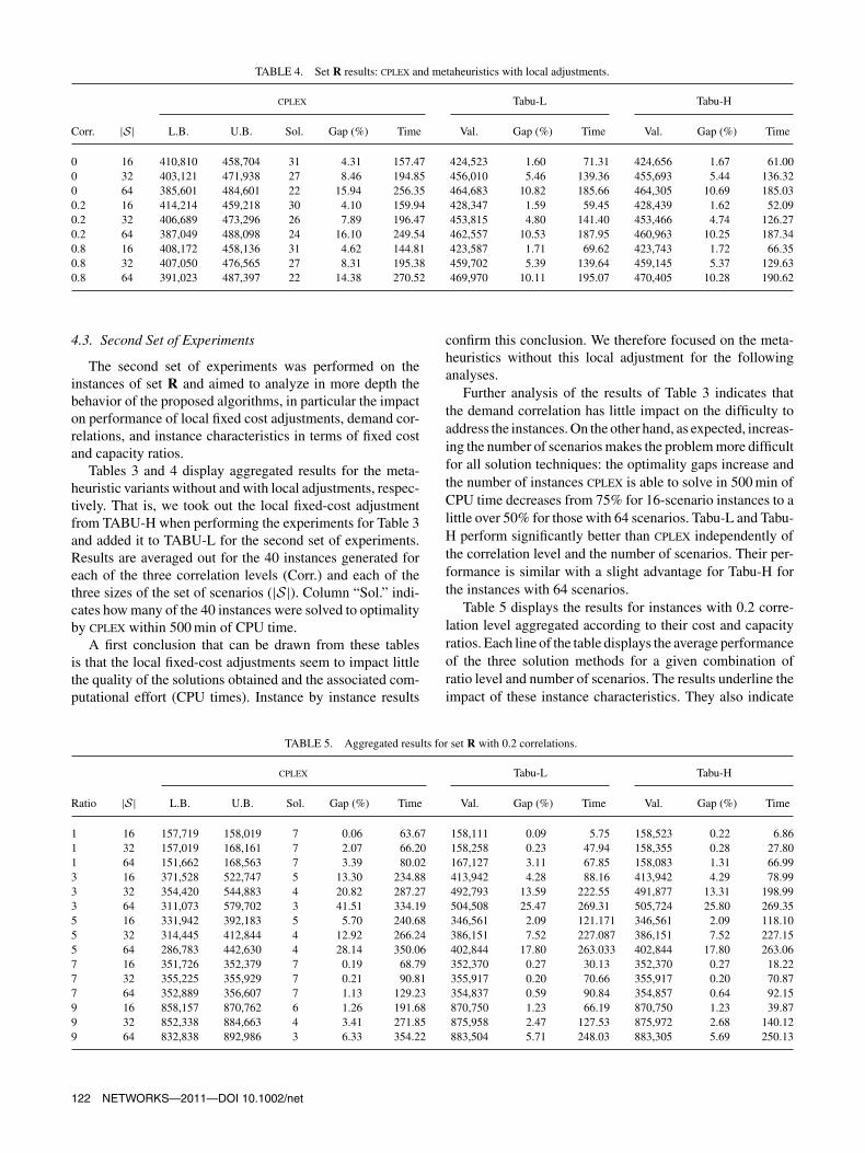
TABLE 4. Set R results: cplex and metaheuristics with local adjustments.

cplex Tabu-L Tabu-H

Corr. |S| L.B. U.B. Sol. Gap (%) Time Val. Gap (%) Time Val. Gap (%) Time

0 16 410,810 458,704 31 4.31 157.47 424,523 1.60 71.31 424,656 1.67 61.000 32 403,121 471,938 27 8.46 194.85 456,010 5.46 139.36 455,693 5.44 136.320 64 385,601 484,601 22 15.94 256.35 464,683 10.82 185.66 464,305 10.69 185.030.2 16 414,214 459,218 30 4.10 159.94 428,347 1.59 59.45 428,439 1.62 52.090.2 32 406,689 473,296 26 7.89 196.47 453,815 4.80 141.40 453,466 4.74 126.270.2 64 387,049 488,098 24 16.10 249.54 462,557 10.53 187.95 460,963 10.25 187.340.8 16 408,172 458,136 31 4.62 144.81 423,587 1.71 69.62 423,743 1.72 66.350.8 32 407,050 476,565 27 8.31 195.38 459,702 5.39 139.64 459,145 5.37 129.630.8 64 391,023 487,397 22 14.38 270.52 469,970 10.11 195.07 470,405 10.28 190.62

4.3. Second Set of Experiments

The second set of experiments was performed on theinstances of set R and aimed to analyze in more depth thebehavior of the proposed algorithms, in particular the impacton performance of local fixed cost adjustments, demand cor-relations, and instance characteristics in terms of fixed costand capacity ratios.

Tables 3 and 4 display aggregated results for the meta-heuristic variants without and with local adjustments, respec-tively. That is, we took out the local fixed-cost adjustmentfrom TABU-H when performing the experiments for Table 3and added it to TABU-L for the second set of experiments.Results are averaged out for the 40 instances generated foreach of the three correlation levels (Corr.) and each of thethree sizes of the set of scenarios (|S|). Column “Sol.” indi-cates how many of the 40 instances were solved to optimalityby cplex within 500 min of CPU time.

A first conclusion that can be drawn from these tablesis that the local fixed-cost adjustments seem to impact littlethe quality of the solutions obtained and the associated com-putational effort (CPU times). Instance by instance results

confirm this conclusion. We therefore focused on the meta-heuristics without this local adjustment for the followinganalyses.

Further analysis of the results of Table 3 indicates thatthe demand correlation has little impact on the difficulty toaddress the instances. On the other hand, as expected, increas-ing the number of scenarios makes the problem more difficultfor all solution techniques: the optimality gaps increase andthe number of instances cplex is able to solve in 500 min ofCPU time decreases from 75% for 16-scenario instances to alittle over 50% for those with 64 scenarios. Tabu-L and Tabu-H perform significantly better than cplex independently ofthe correlation level and the number of scenarios. Their per-formance is similar with a slight advantage for Tabu-H forthe instances with 64 scenarios.

Table 5 displays the results for instances with 0.2 corre-lation level aggregated according to their cost and capacityratios. Each line of the table displays the average performanceof the three solution methods for a given combination ofratio level and number of scenarios. The results underline theimpact of these instance characteristics. They also indicate

TABLE 5. Aggregated results for set R with 0.2 correlations.

cplex Tabu-L Tabu-H

Ratio |S| L.B. U.B. Sol. Gap (%) Time Val. Gap (%) Time Val. Gap (%) Time

1 16 157,719 158,019 7 0.06 63.67 158,111 0.09 5.75 158,523 0.22 6.861 32 157,019 168,161 7 2.07 66.20 158,258 0.23 47.94 158,355 0.28 27.801 64 151,662 168,563 7 3.39 80.02 167,127 3.11 67.85 158,083 1.31 66.993 16 371,528 522,747 5 13.30 234.88 413,942 4.28 88.16 413,942 4.29 78.993 32 354,420 544,883 4 20.82 287.27 492,793 13.59 222.55 491,877 13.31 198.993 64 311,073 579,702 3 41.51 334.19 504,508 25.47 269.31 505,724 25.80 269.355 16 331,942 392,183 5 5.70 240.68 346,561 2.09 121.171 346,561 2.09 118.105 32 314,445 412,844 4 12.92 266.24 386,151 7.52 227.087 386,151 7.52 227.155 64 286,783 442,630 4 28.14 350.06 402,844 17.80 263.033 402,844 17.80 263.067 16 351,726 352,379 7 0.19 68.79 352,370 0.27 30.13 352,370 0.27 18.227 32 355,225 355,929 7 0.21 90.81 355,917 0.20 70.66 355,917 0.20 70.877 64 352,889 356,607 7 1.13 129.23 354,837 0.59 90.84 354,857 0.64 92.159 16 858,157 870,762 6 1.26 191.68 870,750 1.23 66.19 870,750 1.23 39.879 32 852,338 884,663 4 3.41 271.85 875,958 2.47 127.53 875,972 2.68 140.129 64 832,838 892,986 3 6.33 354.22 883,504 5.71 248.03 883,305 5.69 250.13


that the instances that are the most difficult to address are notthose with the highest fixed cost and capacity ratio, an obser-vation often made for deterministic CMND problems e.g.,Refs. [4] and [5] but rather those with intermediate ratios.A possible explanation for this behavior may come from thehigher number of “almost” equivalent optimal designs thatexist for such intermediary deterministic CMND instancesthan for instances with low (when the multicommodity flowaspect of the problem dominates) or high (the arc selectiondecisions dominate and there are few equivalent optimal solu-tions) ratios. In a stochastic context with random demandparameters, such instances may display broader differencesamong scenarios requiring more effort to identify an overallsatisfactory, hopefully optimal, solution.

The proposed metaheuristic, using either the Lagrangean-based or the heuristic fixed-cost adjustment, perform verywell overall and, particularly, on the most difficult classes ofinstances. Optimality gaps appear high for these instances,but the well-documented weakness of the CMND lowerbound contributes for a large part to these figures. It isnoticeable that the proposed metaheuristic is able to iden-tify the optimal solution when cplex finds it and doesso with less computational effort. The performance of themetaheuristic is even more impressive when more difficultinstances are addressed, both the gaps and the computationalefforts being significantly reduced. To conclude, the proposedmetaheuristic approach appears very promising to address thefixed-cost capacitated multicommodity stochastic networkdesign problem.

5. CONCLUSIONS

In this article, we have addressed the stochastic fixed-cost capacitated multicommodity network design problemand proposed a two-stage stochastic programming formula-tion where design decisions make up the first stage, while anetwork recourse, providing additional capacity at high costbetween each pair of origin-destination nodes, distributes thecommodities according to observed demands in the secondstage.

We proposed a metaheuristic solution strategy inspired bythe progressive hedging idea to address the S-CMND. Theproposed metaheuristic was shown to be very efficient whenaddressing a large set of diverse stochastic CMND problems,outperforming in both solution quality and computationaleffort the latest version of well-known commercial solveraddressing directly the multiscenario formulations.

A number of research avenues appear promising toenhance the proposed metaheuristic framework. The explo-ration of alternate mechanisms to modify the fixed costsin searching for the overall solution is one such avenue. Adifferent one would explore the utilization of the memorymechanisms typical of tabu search metaheuristics to identifyparts of the solution space where the search could either beintensified or diversified. A third promising research avenue

consists in combining elements from exact solution meth-ods (e.g., cuts) to the metaheuristic framework. Last but notleast, more advanced parallel solution strategies should beexplored to, on the one hand, increase the size of the probleminstances that one may address and, on the other hand, pro-vide the means for more advanced scenario decompositionand search cooperation mechanisms. We plan to investigatethese avenues in the near future.

Acknowledgments

While working on this project, TGC was the NSERCIndustrial Research Chair in Logistics Management, ESGUQAM, and Adjunct Professor with the Department ofComputer Science and Operations Research, Université deMontréal, and the Department of Economics and BusinessAdministration, Molde University College, Norway. TGC,XF, MG, and WR were also members of CIRRELT—theInteruniversity Research Centre on Enterprise Networks,Logistics and Transportation.

REFERENCES

[1] J.R. Birge and F. Louveaux, Introduction to StochasticProgramming, Springer, New York Berlin Heidelberg, 1997.

[2] T.G. Crainic, Network design in freight transportation, Eur JOper Res 122 (2000), 272–288.

[3] T.G. Crainic and K. Kim, “Intermodal Transportation,”Transportation, volume 14 of Handbooks in OperationsResearch and Management Science, chapter 8, In C. Barnhartand G. Laporte (Editors), North-Holland, Amsterdam, 2007,pp. 467–537.

[4] T.G. Crainic, B. Gendron, and G. Hernu, A slope scal-ing/lagrangean perturbation Heuristic with long-term mem-ory for multicommodity capacitated fixed-charge networkdesign, J Heuristics 10 (2004), 525–545.

[5] I. Ghamlouche, T.G. Crainic, and M. Gendreau, Cycle-basedneighbourhoods for fixed-charge capacitated multicommod-ity network design, Oper Res 51 (2003), 655–667.

[6] K.K. Haugen, A. Løkketangen, and D. Woodruff, Progressivehedging as a meta-heuristic applied to stochastic lot-sizing,Eur J Oper Res 132 (2001), 116–122.

[7] A. Hoff, A.-G. Lium, A. Løkketangen, and T.G. Crainic, Ametaheuristic for stochastic service network design, J Heuris-tics 16 (2010), 653–679.

[8] K. Høyland, M. Kaut, and S.W. Wallace, A heuristic formoment-matching scenario generation, Comput Optim Appl24 (2003), 169–185.

[9] L.M. Hvattum and A. Løkketangen, Using scenario treesand progressive hedging for stochastic inventory routingproblems, J Heuristics 15 (2009), 527–557.

[10] P. Kall and S. Wallace, Stochastic Programming, Wiley,Chichester, NY, 1994.

[11] A.-G. Lium, T.G. Crainic, and S.W. Wallace, A study ofdemand stochasticity in service network design, TransportSci 43 (2009), 144–157.


[12] A. Løkketangen and D. Woodruff, Progressive hedgingand tabu search applied to mixed integer (0,1) multistagestochastic programming, J Heuristics 2 (1996), 111–128.

[13] D.G. Luenberger and Y. Ye, Linear and Nonlinear Program-ming, 3rd edition, Springer, New York, 2008.

[14] T.L. Magnanti and R. Wong, Network design and trans-portation planning: Models and algorithms, Transport Sci 18(1986), 1–55.

[15] M. Minoux, Network synthesis and optimum network designproblems: Models, solution methods and applications, Net-works 19 (1986), 313–360.

[16] R.T. Rockafellar and R.J.-B. Wets, Scenarios and policyaggregation in optimization under uncertainty, Math OperRes 16 (1991), 119–147.

[17] S.W. Wallace, Decision making under uncertainty: Is sensi-tivity analysis of any use?, Oper Res 48 (2000), 20–25.


Documents

Progressive hedging-based metaheuristics for stochastic network design