Réduction de Modèles à l’Issue de la Réduction de Modèles à l’Issue de la

Théorie CinétiqueThéorie Cinétique

Francisco CHINESTA Francisco CHINESTA

LMSP – ENSAM ParisLMSP – ENSAM Paris

Amine AMMARAmine AMMAR

Laboratoire de Rhéologie, INPG Laboratoire de Rhéologie, INPG GrenobleGrenoble

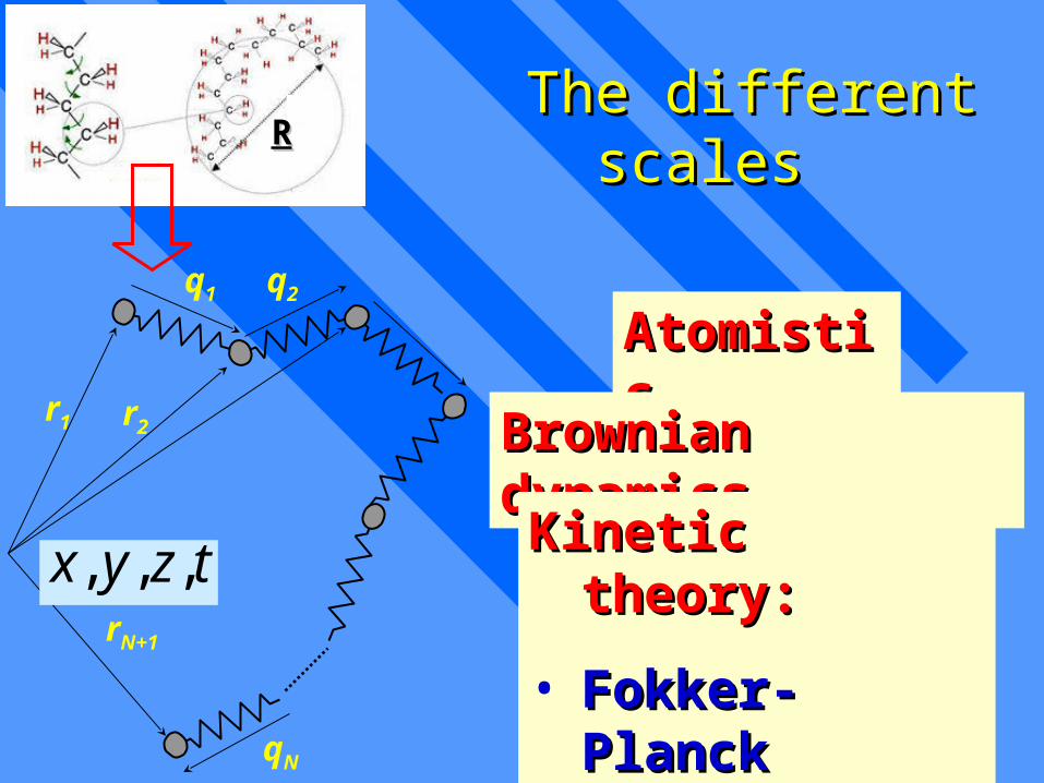
The different scalesThe different scales

r1 r2

rN+1

q1 q2

qN

RR

tzyx ,,,

AtomisticAtomistic

Brownian dynamicsBrownian dynamics

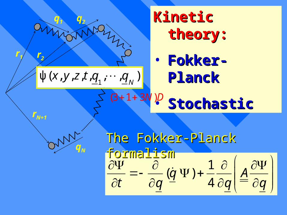
Kinetic theory:Kinetic theory:

• Fokker-PlanckFokker-Planck

• StochasticStochastic

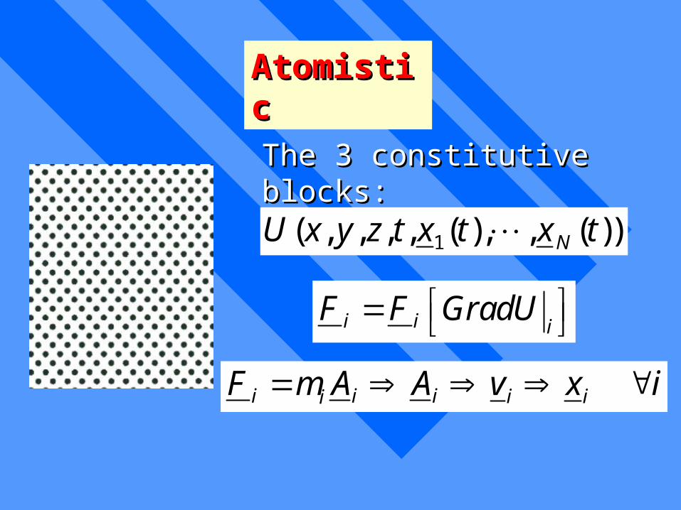
AtomisticAtomistic

1( , , , , ( ), , ( ))NU x y z t x t x t

i i iF F GradU

i i i i iiF m A A v x i

The 3 constitutive blocks:The 3 constitutive blocks:

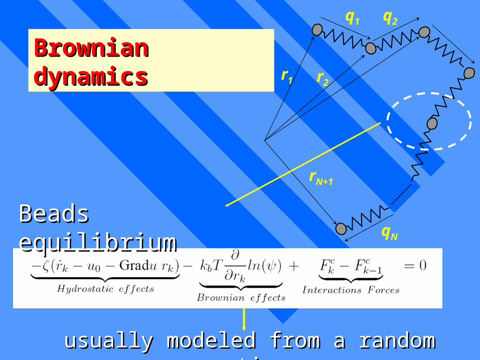
Brownian dynamicsBrownian dynamicsr1 r2

rN+1

q1 q2

qN

usually modeled from a random motionusually modeled from a random motion

Beads equilibriumBeads equilibrium

r1 r2

rN+1

q1 q2

qN

Kinetic theory:Kinetic theory:

• Fokker-PlanckFokker-Planck

• StochasticStochastic),,,,,,(ψ1 N

qqtzyx

(3 1 3 )N D

1( )

4q A

t q q q

The Fokker-Planck formalismThe Fokker-Planck formalism

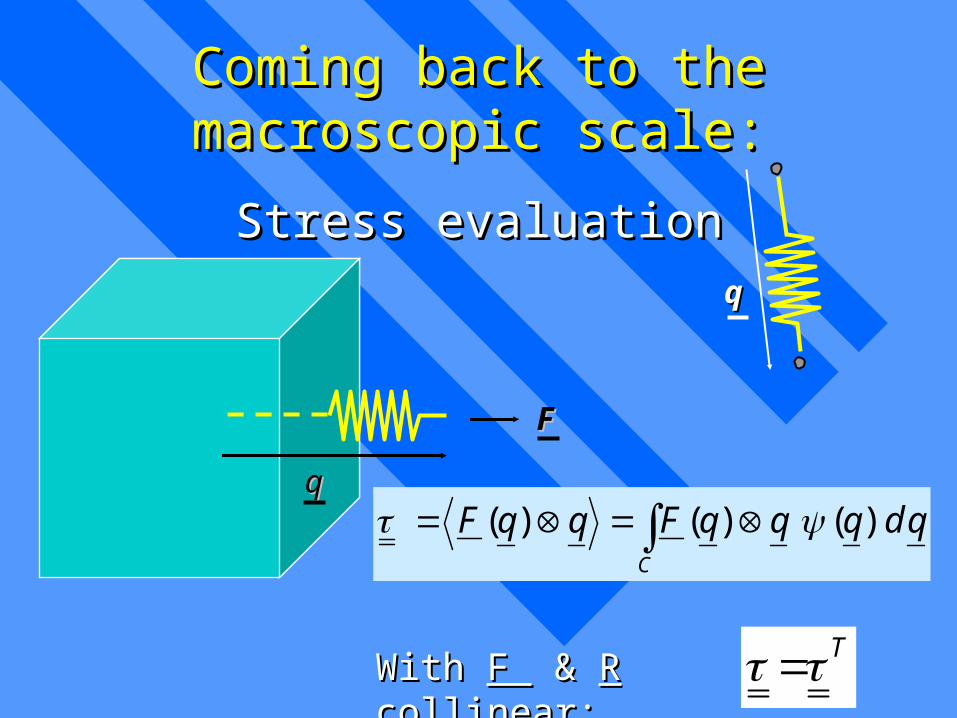
Coming back to the macroscopic scale:Coming back to the macroscopic scale:

Stress evaluationStress evaluation

qqFF( ) ( ) ( )

C

F q q F q q q dq

With With F F & & RR collinear collinear:: T

qq

FF

Solving the deterministic Solving the deterministic Fokker-Planck equationFokker-Planck equation

Two new model Two new model reduction approachesreduction approaches

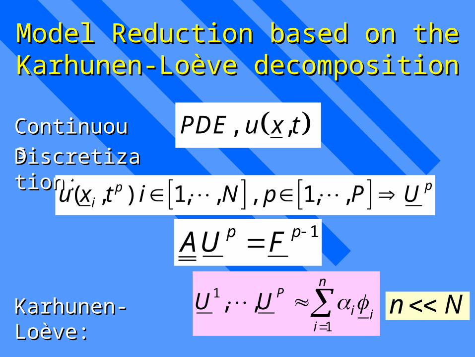
Model Reduction based on the Model Reduction based on the Karhunen-Loève decompositionKarhunen-Loève decomposition

, ,PDE u x t

( , ) 1, , , 1, , ppiu x t i N p P U

1 pp FUA

n N

Continuous:Continuous:

Discretization:Discretization:

1

1

, ,n

Pi i

i

U U

Karhunen-Loève:Karhunen-Loève:

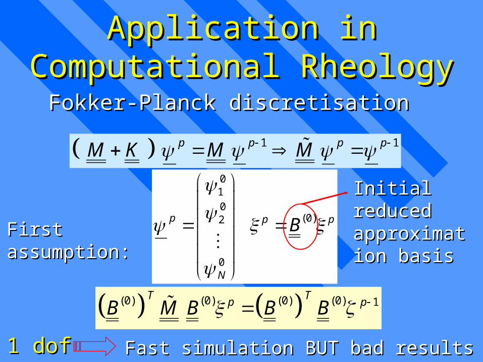
Application in Computational Application in Computational RheologyRheology

1 1 p p p pM K M M

Fokker-Planck discretisation Fokker-Planck discretisation

010

(0)2

0

p p p

N

B

(0) (0) (0) (0) 1 T T

p pB M B B B

1 dof !1 dof !

First assumption:First assumption:

Initial reduced Initial reduced approximation approximation basisbasis

Fast simulation BUT bad results expectedFast simulation BUT bad results expected

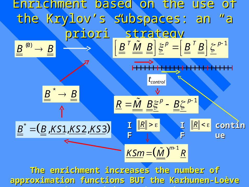
Enrichment based on the use of the Krylov’s Enrichment based on the use of the Krylov’s subspaces: an “a priori” strategysubspaces: an “a priori” strategy

controlt

1mKSm M R

IFIF R IFIF R continuecontinue

1 p pR M B B

1 T p T pB M B B B

* , 1, 2, 3B B KS KS KS

(0)B B

*B B

The enrichment increases the number of approximation The enrichment increases the number of approximation functions BUT the Karhunen-Loève decomposition reduces it functions BUT the Karhunen-Loève decomposition reduces it

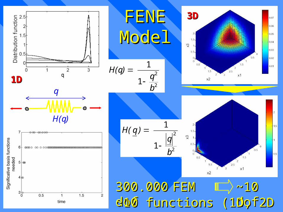
FENE FENE ModelModel

300.000300.000 FEM dofFEM dof ~10~10 dofdof~10 functions (1D, 2D or 3D)~10 functions (1D, 2D or 3D)

3D3D

2

2

1

1

H( q )q

b

2

2

1 1

H(q)qb

1D1D

q

H(q)

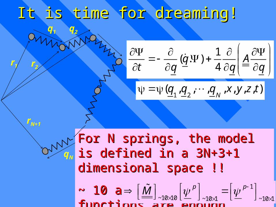
It is time for dreamingIt is time for dreaming!!

qA

qq

qt 4

1).(

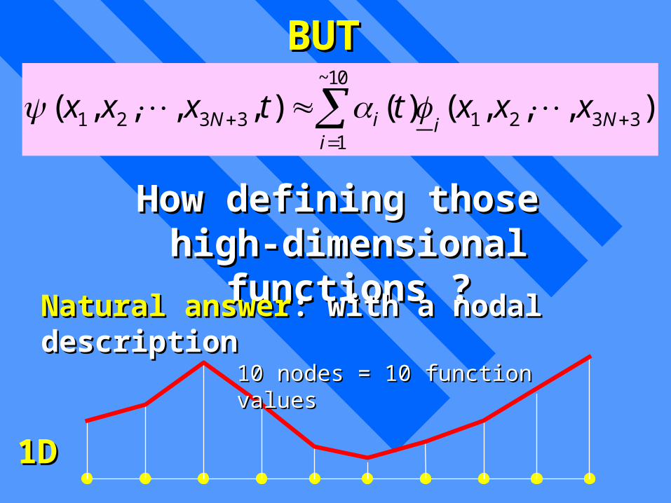
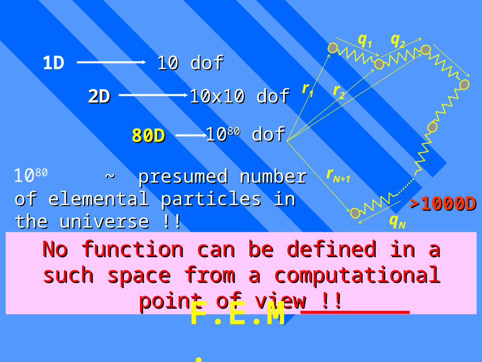
For N springs, the model is defined For N springs, the model is defined in a 3in a 3NN+3+1 dimensional space !! +3+1 dimensional space !!

~ 10 approximation functions are ~ 10 approximation functions are enoughenough

),,,,,,,(21

tzyxqqqN

r1 r2

rN+1

q1 q2

qN

1

~10 10 ~10 1 ~10 1

p pM

BUTBUT ~10

1 2 3 3 1 2 3 31

( , , , , ) ( ) ( , , , )N i Nii

x x x t t x x x

How defining those How defining those high-dimensional functions ?high-dimensional functions ?

Natural answerNatural answer: with a nodal description: with a nodal description

1D1D

10 nodes = 10 function values10 nodes = 10 function values

1D

2D2D

>1000D>1000D

r1 r2

rN+1

q1 q2

qN

80D80D

10 dof10 dof

10x10 dof10x10 dof

10108080 dof dof

No function can be defined in a such space from No function can be defined in a such space from a computational point of view !!a computational point of view !!

F.E.M.

1080 ~ presumed number of~ presumed number of elemental particles in the universe !!elemental particles in the universe !!

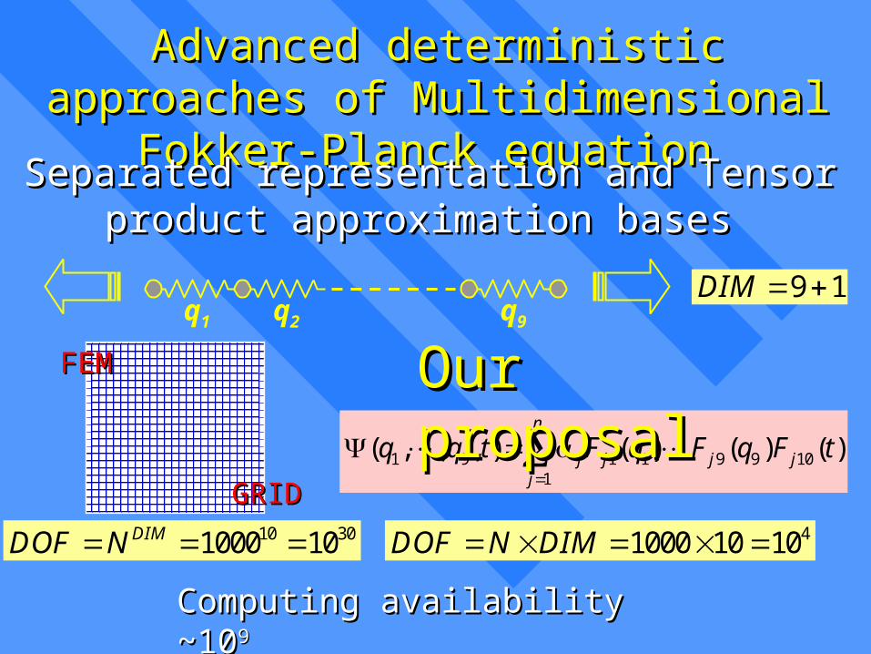
Advanced deterministic approaches of Advanced deterministic approaches of Multidimensional Fokker-Planck equationMultidimensional Fokker-Planck equation

Separated representation and Tensor product Separated representation and Tensor product approximation bases approximation bases

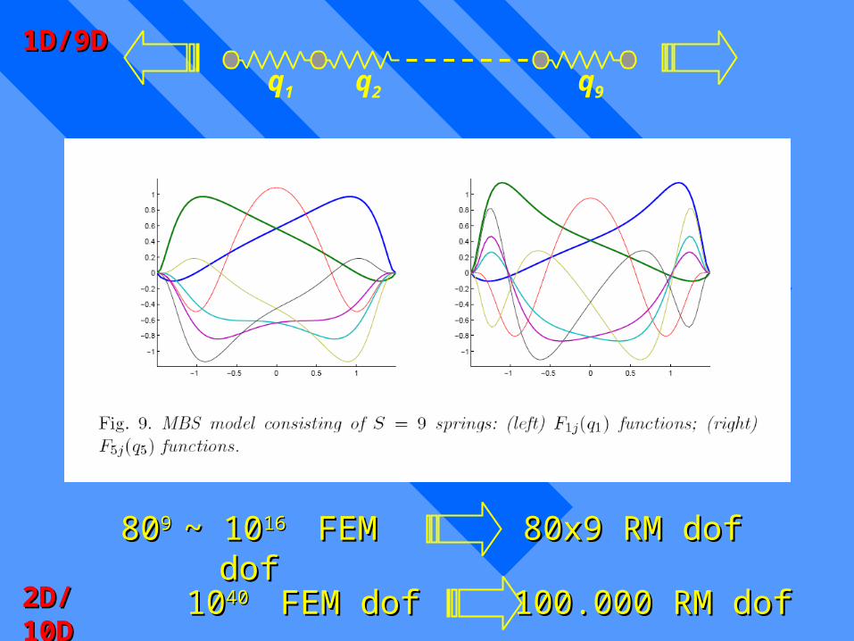
q1 q2 q9

FEMFEM

GRIDGRID10 301000 10DIMDOF N

1 9 1 1 9 9 101

( , , , ) ( ) ( ) ( )n

j j j jj

q q t F q F q F t

Our Our proposalproposal

9 1DIM

41000 10 10DOF N DIM

Computing availabilityComputing availability ~10 ~109 9

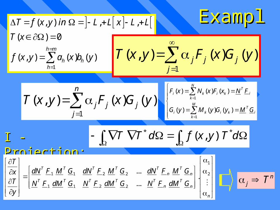
ExamplExamplee

1

( , ) , ,

( ) 0

( , ) ( ) ( )h m

h hh

T f x y in L L x L L

T x

f x y a x b y

1

( , ) ( ) ( )j j jj

T x y F x G y

1

( , ) ( ) ( )n

j j jj

T x y F x G y

1

1

( ) ( ) ( )

( ) ( ) ( )

NT

ii k i kk

MT

ii k i kk

F x N x F x N F

G y M y G y M G

I - Projection:I - Projection:* * ( , ) T T d f x y T d

1

1 21 2 2

1 21 2

....

...

T T T T T Tn n

T T T T T Tn n

n

TdN F M G dN F M G dN F M Gx

T N F dM G N F dM G N F dM Gy

n

j T

1

( , ) ( ) ( )n

j j jj

T x y F x G y

1

1

n

n

RF

R

SG

S

* * ( , ) T T d f x y T d

(1, )

1 (1, )

. . 0

. 0 .

T T T Tnj j q

j T T T Tj j j p

TdN F M G M S dN Rx

T SN F dM G N R dMy

***

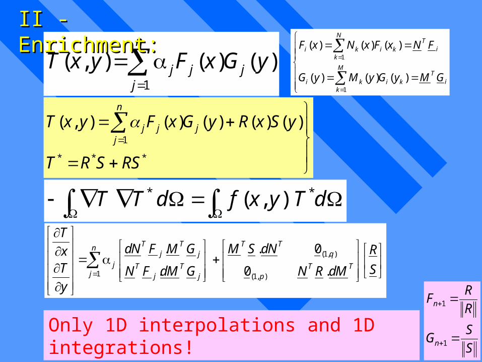
1

)()()()(),(

RSSRT

ySxRyGxFyxTn

jjjj

1

1

( ) ( ) ( )

( ) ( ) ( )

NT

ii k i kk

MT

ii k i kk

F x N x F x N F

G y M y G y M G

Only 1D interpolations and 1D integrations!

II - Enrichment:II - Enrichment:

q1 q2

q1 q2 q9

80809 9 ~ 10~ 1016 16 FEM dof FEM dof 80x9 RM dof80x9 RM dof

101040 40 FEM dof FEM dof 100.000 RM dof100.000 RM dof

1D/9D1D/9D

2D/10D2D/10D

Solving the Stochastic Solving the Stochastic representation of the representation of the

Fokker-Planck equationFokker-Planck equation

New efficient solversNew efficient solvers

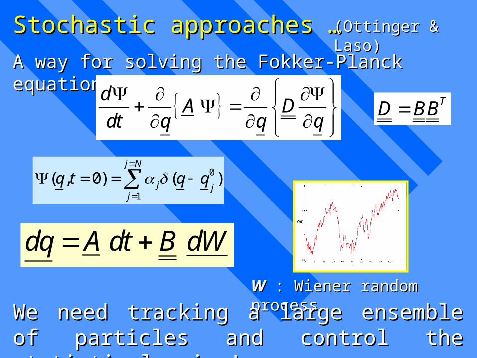
Stochastic approaches …Stochastic approaches …

A way for solving the Fokker-Planck equation:A way for solving the Fokker-Planck equation:

(Ottinger & Laso)(Ottinger & Laso)

d

A Ddt q q q

dq A dt B dW WW : Wiener random process : Wiener random process

We need tracking a large ensemble of particles We need tracking a large ensemble of particles and control the statistical noise!and control the statistical noise!

0

1

( , 0) ( )j N

j jj

q t q q

TD BB

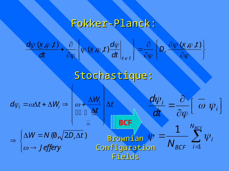
Fokker-Planck:Fokker-Planck:

, ,

( , , ) ( , , )( , , ) r

x t

d x t d x tx t D

dt dt

Stochastique:Stochastique:

(0, 2 )

ii i

r

Wd t W t

t

W N D t

Jeffery

BCF

1

1 BCF

ii

N

iiBCF

d

dt

N

Brownian Brownian Configuration Configuration

FieldsFields

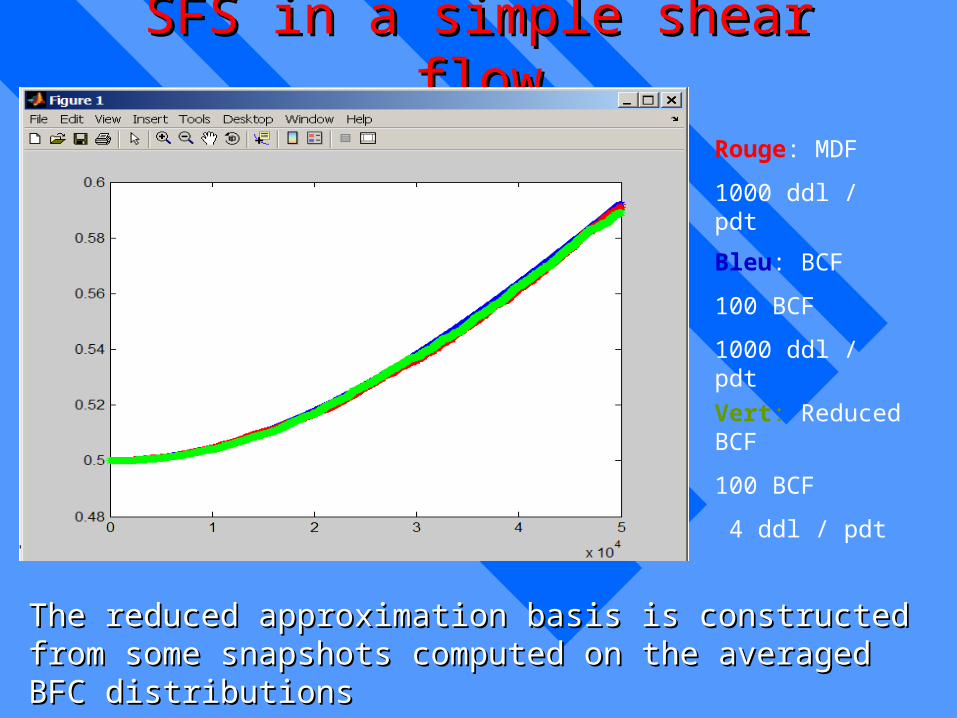
SFS in a simple shear flowSFS in a simple shear flow

Rouge: MDF

1000 ddl / pdt

Bleu: BCF

100 BCF

1000 ddl / pdt

Vert: Reduced BCF

100 BCF

4 ddl / pdt

a11

t

The reduced approximation basis is constructed from some The reduced approximation basis is constructed from some snapshots computed on the averaged BFC distributionssnapshots computed on the averaged BFC distributions

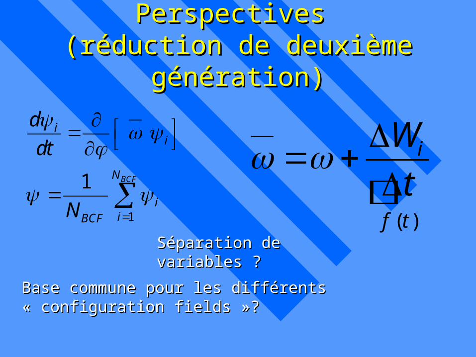
Perspectives Perspectives (réduction de deuxième génération)(réduction de deuxième génération)

1

1 BCF

ii

N

iiBCF

d

dt

N

( )

i

f t

W

t

Séparation de variables ?Séparation de variables ?

Base commune pour les différents « configuration fields »?Base commune pour les différents « configuration fields »?