Time-periodic solutions of multidimensional Hamilton systems

Volume 160B, number 6 PHYSICS LETTERS 17 October 1985

TIME-PERIODIC SOLUTIONS OF MULTIDIMENSIONAL HAMILTON SYSTEMS

E. C AUR I ER Centre de Recherches Nuclbaires et Unioersitb Louis Pasteur de Strasbourg Groupe de Physique Nuclbaire Thborique, BP 20, 67037 Strasbourg Cedex, France

M. PLOSZAJCZAK 1 Niels Bohr Institut, Blegdamsoej 17, DK-2100 Copenhagen O, Denmark

and

S. DROZDZ; 1 lnstitut flir Kernphysik, D-5170 Jiilich, West Germany

Received 14 March 1985; revised manuscript received 7 June 1985

A simple method is proposed to determine the time-periodic solutions of a non-separable hamiltonian system in the regular domain of a phase space. This method is applied for the quantization of gauge-invariant time-dependent Hartree-Fock solutions for the deformed oscillator (DO) and SU(3) models. Energies of the quantized states and the "collective" variables for decoupled modes are compared with the corresponding RPA results.

An application of the hamiltonian dynamics for bounded quantal systems requires the formulation of appropriate boundary conditions which is provided, for instance, by the regularity and single-valuedness (RSV) principle for gauge- invariant solutions of the SchriSdinger time-depen- "dent variational principle [1,2]. This method can be~applied in any manifold of the Hilbert space [3], both for the bound state problem [1,4] and for tunneling [5]. It provides a variational approach to the quantum dynamics and as such, it depends mainly on the chosen variational manifold { if(q, p)} for canonical conjugate, classical variables q and p. The RSV method underlines particularly the role of q, p as labels of the evolving wave function and the interpretation of the expectation value Je'(q, p ) = (if(q, P)I Hli(q, P)) of the quantal many-body hamiltonian as the classical hamiltonian [6]. Consequently, the

SchriSdinger time-dependent variational principle yields quite naturally the Hamilton equations for the time-development of q, p and henc e if (q, p) . Increasing the number of labels q, p is equivalent to a gradual changing from a classical to a quantum theory. Finally, in the full Hilbert space, one arrives at the time-dependent SchrSdinger equation and the RSV quantization prescription yields all the SchriSdinger eigenstates and only them [1,4]. The details of the RSV quantization method can be found in our earlier works [1,5,7]. Here we remind only that the relation between labels q, p and a phase-determiried gauge- invariant wave function ifo(r; q, p ) is regular and single-valued if for any closed trajectory C O

~cy 'dq= 2*rn°h' n o=O,1 . . . . . (1)

1 On leave of absence from the Institute of Nuclear Physics, PL-31-342, Cracow, Poland.

This property is assumed to hold for any physical bound state and can be rewritten in the form of

0370-2693/85/$ 03.30 © Elsevier Science Publishers B.V. (North-Holland Physics Publishing Division) 357

Volume 160B, number 6 PHYSICS LETTERS 17 October 1985.

a quantization condition

I,=(2*) i d' dq=',h,

n , = 0 , 1 . . . . . i = 1 . . . . ,N, (2)

for components of the action integral I = [ I 1 . . . . . IN] where 2N is the dimensionality of the label space (parametric region). This, however, is possible if one can find N topologically independent basic closed curves (Ci): C o = ~N=IMiC i for [M 1 . . . . . MN] being a set of integer numbers. One should notice that in contrast to quasi-classical methods [8], the quantization path in the RSV quantization method is constructed in the space of phase-determined wave functions and not in the classical configuration space. Consequently, the Maslov index [9] does not enter into expressions (1), (2) and the lowest quantized solutions I (o = [ I 1 = 0 . . . . . I , = n,h . . . . . I N = 0 ] ( i = 1 . . . . . N )

should be time periodic. Those "stationary" solutions are particularly interesting since they offer a generalization of RPA modes for infinitesimal oscillations.

Our discussion in this work is devoted to the presentation of a simple and practical approach towards selecting periodic trajectories which represent the topologically independent closed circuits on the invariant torus. Obviously, we anticipate the existence of invariant toil at least in a part of the parametric region (q, p }. Kolmogorov-Arnold-Moser and Nekhoroshev theorems [10,11] ensure their existence for small non-integral conservative perturbations, i.e. at low excitation energies. In practice this is sufficient because most of the higher lying states cannot be separated out of the continuum.

In our previous paper [12], we have constructed decoupled or least-coupled variables of a hamiltonian system by initializing the collective motion through the velocity field at the equilibrium point q = qeq, P = 0 and calculating the corresponding action integrals at the Poincar6 surfaces of section. For each mode j in the decoupled canonical variables (q;, p;, i = 1 . . . . . N), the ratio of action integrals I J I j has to be equal zero for all k #: j . In a more general case of non-separable hamiltonian, we have been looking in ref. [12] for the

least-coupled variables of the system by minimizing the ratios I k / I j ( k -~ j , k = 1 . . . . . N ) obtained for various initial velocity fields or, equivalently, for differently defined canonical variables. At low excitations, i.e. for nearly harmonic vibrations, this method was siaccessful in finding decoupled modes of a time-dependent deformed oscillator model [12]. However, at higher excitations the decoupled variables could not be found, even though the coupling between modes was strongly reduced. Below we show that the choice of the equilibrium deformation qeq as an initial evolution point was the main reason for this failure. We shall also illustrate this observation in two different dynamical systems.

In ref. [12] we have used the Poincar6 surfaces of section to estimate the coupling of modes. This restricts somehow the applicability of the method because the surfaces of section cannot be calcu- lated exactly and have some "width" already in N = 3 hamiltonian systems. To avoid this dif- ficulty, we have proposed in ref. [12] an iterative procedure in which the N-dimensional (N > 2) canonical transformations from original variables to supposedly less coupled ones, are replaced by a series of two-dimensional canonical transformations. To find in this way an optimal N-dimensional transformation towards least-coupled variables, one should repeat this iterative scheme a few times, which turns out to be computationally inefficient already for N > 5.

In this letter we propose a different method which does not use the Poincar6 sections of an invariant torus in finding the least-coupled variables. Moreover, for each excitation energy E* the collective motion is initiated with p = 0, i.e. by choosing initial values of the collective coordinate on the equi-energy surface .~(q, p = 0) = (~(q , p = 0)lnltk(q, p = 0)) = E*, where ~(q, p ) is the variational wave function and H is a many-body hamiltonian. This method is based on the following observation. The trajectory region of a non-degenerate dynamical system sufficiently close to its equilibrium point (q = qeq, P = 0) exhibits well-behaved caustics which touch the energy surface .,~(q, p = 0) = E * in 2Ndifferent points. These points coalesce in decoupled variables for modes I (i) = [11 = 0 . . . . . //4= 0 . . . . . I N =

358


0], i = 1 . . . . . N and, consequently, each of these modes is represented on .,'if(q, p = 0) by a pair of points. These are the two turning points of a time-periodic trajectory joining the two "opposite" caustics without being reflected from other caustics. Hence, the construction of N decoupled modes reduces to the problem of finding N pairs of such points as initial conditions. Obviously, for non-separable systems our aim is to find N pairs of initial conditions (initial points) on o~ff(q, p = 0) such that the resulting quasiperiodic trajectory for each of them comes back as close as possible to the initial point after each two subsequent turn- ings.

The numerical procedure of finding the initial points on o~ff(q, p = 0) goes as follows. We begin at low excitation energy E(T ) by selecting the reference initial points on o~ff(q, p = 0) = E(~) which for example can be found by determining RPA modes. The position of each point on o~ff(q, p = 0) = E(T ) can be conveniently assigned by N - 1 polar angles [81 . . . . . ON_I]. Then keeping these angles unchanged the excitation energy is increased E(~) ~ E(~) = E(~) + AE and we determine a new initial point on .,'if(q, p = 0) = E(~). In general, these points may not give rise to the least-coupled modes and one should try to find better points. For that, in the neighbourhood of each reference point we initiate the evolution in a few mesh points. For each of these evolutions we calculate the difference mi, f = tq(i)- q(t)l of initial and final q-values at the first minimum of this quantity, i.e. after one oscillation. Obviously, if Ai,~ = 0 then P(i) =Pu) -- 0 and we have found a decoupled variable. However, in general P( i )4 : p ( f ) and the final point q(t) is situated at the nearby caustic line for which one of the components of the momentum p is equal zero. Minimizing the function A i, f around each reference point sep- arately, one can find easily an optimal set of angles [01 . . . . . ON_I] for each mode.

For these optimized modes j ( = 1 . . . . . N) we now calculate the action integrals

= (2or)-1 f q m p . dq, I ( J ) (3) q(i)

and check whether they satisfy the RSV quantization condition. For those that do not obey the

RSV condition, we change the excitation energy and the newly found optimal angles provide us with the necessary points of reference. We con- tinue with this numerical procedure until the quantized energy of each decoupled or least- coupled mode is found. An identification of "collective" variables by comparison with those at infinitesimal excitations is straightforward provided the variation of optimal initial points with energy is continuous. This continuity is ensured if the invariant torus exists and, moreover, if it can be obtained by continuous deformations of the invariant torus at infinitesimal excitations. One should remember again that we select only those trajectories which approximately close after one oscillation. In this way, we can be sure that the decoupled modes found, represent topologi- caUy independent basic closed curves on the invariant torus.

Typical examples of periodic trajectories, as obtained using the above method, are shown in fig. 1. The upper picture shows coupled x-, z-shaped oscillations of 8Be which are described using the T D H F approach for a deformed oscillator (DO) model and the Bl-force [14]. Details of this model can be found in refs. [7,12]. Here, we only remind that the variational wave packets are given by the Slater determinant of single-particle states which are (nxny nz)-eigenfunctions of the harmonic oscillator potential. The single-particle wave functions

(Xlnx) =/¢nx Xexp(-X[px(t)+i~rx(t)](x2/b(~°))} (4)

are boosted and the time-evolution of the wave packet is parametrized by pi,~rr Canonical variables are obtained by a transformation:

qi = pf -1 , Pi = gi"a'i,

i = x, y, z; h = b i = 1, (5)

where A

K , = ( A + 2 N , - 1 ) / 8 , N~= E n, k = l

goes over occupied single-particle states. For the sake of convenience, we have redefined those variables so that the ground-state equilibrium

359


I Q 2 ~ -

i -4.0

Q !

2 d -

°Be

-01.6 01.0 OIS 41.0 41.6 21.0 21.6 $1.0 I

Qt

X--I0 to

d-

d-

N d-

o d"

t~

?

,e I

~o'.2 -o'.i d.o o'., o'.2 o'., Q I

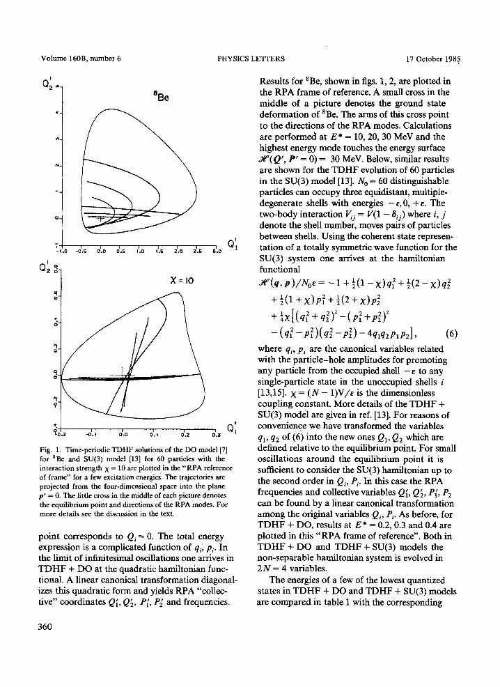
Fig. 1. Time-periodic TDHF solutions of the DO model [7] for 8Be and SU(3) model [13] for 60 particles with the interaction strength X = 10 are plotted in the " R P A reference of frame" for a few excitation energies. The trajectories are projected from the four-dimensional space into the plane p ' = 0. The little cross in the middle of each picture denotes the equilibrium point and directions of the RPA modes. For more details see the discussion in the text.

point corresponds to Q~ = 0. The total energy expression is a complicated function of q f, p~. In the limit of infinitesimal oscillations one arrives in T D H F + DO at the quadratic hamiltonian functional. A linear canonical transformation diagonal- izes this quadratic form and yields RPA "collective" coordinates Qi, Q~, P{, P~ and frequencies.

Results for 8Be, shown in figs. 1, 2, are plotted in the RPA frame of reference. A small cross in the middle of a picture denotes the ground state deformation of 8Be. The arms of this cross point to the directions of the RPA modes. Calculations are performed at E* = 10, 20, 30 MeV and the highest energy mode touches the energy surface 5¢d(Q', P ' = 0) = 30 MeV. Below, similar results are shown for the T D H F evolution of 60 particles in the SU(3) model [13]. N O = 60 distinguishable particles can occupy three equidistant, multiple- degenerate shells with energies - e , 0, + e. The two-body interaction V/j = V(1 - 8q) where i, j denote the shell number, moves pairs of particles between shells. Using the coherent state represen- tation of a totally symmetric wave function for the SU(3) system one arrives at the hamiltonian functional

.g~(q, p )/Noe = - 1 + ½(1 - x)q 2 + ½(2 - x)q 2 + 1(1 + X)p 2+½(2 + X ) p 2

+ 1x[(q? + q~)2_(p~ + p~)~

- (q~-p21)(q~-p~)-4qlq2plp2] , (6)

where q;, p~ are the canonical variables related with the particle-hole amplitudes for promoting any particle from the occupied shell - e to any single-particle state in the unoccupied shells i [13,15]. X = (N - 1)V/e is the dimensionless coupling constant. More details of the T D H F + SU(3) model are given in ref. [13]. For reasons of convenience we have transformed the variables qx, q2 of (6) into the new ones Q1, Q2 which are defined relative to the equilibrium point. For small oscillations around the equilibrium point it is sufficient to consider the SU(3) hamihonian up to the second order in Q~, Pv In this case the RPA frequencies and collective variables Q~, Q~, P{, P2 can be found by a linear canonical transformation among the original variables Qi, Pi. As before, for T D H F + DO, results at E* = 0.2, 0.3 and 0.4 are plotted in this "RP A frame of reference". Both in T D H F + DO and T D H F + SU(3) models the non-separable hamiltonian system is evolved in 2N = 4 variables.

The energies of a few of the lowest quantized states in T D H F + DO and T D H F + SU(3) models are compared in table 1 with the corresponding

360

Volume 160B, number 6

o' o_

"1 - 1.0 -Or.5 O'.C 01.5

8Be

I

~1.0 ~1.~ 21.0 21,S ~1. 0 QI

PHYSICS LETTERS 17 October 1985

I

Q2 -"- X =10

ul;

I

2 - 0 1 O 0 O I 0 2 0'.11 QI

I m

Y I00

N

a

¢

' * ,s -"ho -o:o~ o~oo o~o~ oho o:,s oho Q't

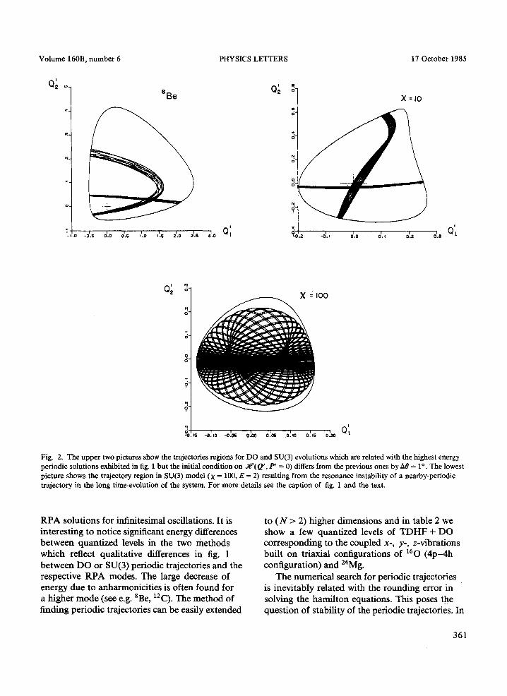
Fig. 2. The upper two pictures show the trajectories regions for DO and SU(3) evolutions which are related with the highest energy periodic solutions exhibited in fig. 1 but the initial condition on ,,~(Q', P' = 0) differs from the previous ones by A# = 1 °. The lowest picture shows the trajectory region in SU(3) model (X = 100, E = 2) resulting from the resonance instability of a nearby-periodic trajectory in the long time-evolution of the system. For more details see the caption of fig. 1 and the text.

R P A solutions for infinitesimal oscillations. It is interesting to notice significant energy differences between quant ized levels in the two methods which reflect qualitative differences in fig. 1 between D O or SU(3) periodic trajectories and the respective R P A modes. The large decrease of energy due to anhannonici t ies is often found for a higher m o d e (see e.g. abe, 12C). The method of finding periodic trajectories can be easily extended

to ( N > 2) higher dimensions and in table 2 we show a f e w quantized levels of T D H F + D O cor responding to the coupled x-, y-, z-vibrations buil t on triaxial configurations of 160 ( 4 p - 4 h configurat ion) and 24Mg.

The numerical search for periodic trajectories is inevitably related with the rounding error in solving the hami l ton equations. This poses the ques t ion of stability of the periodic trajectories. In

361


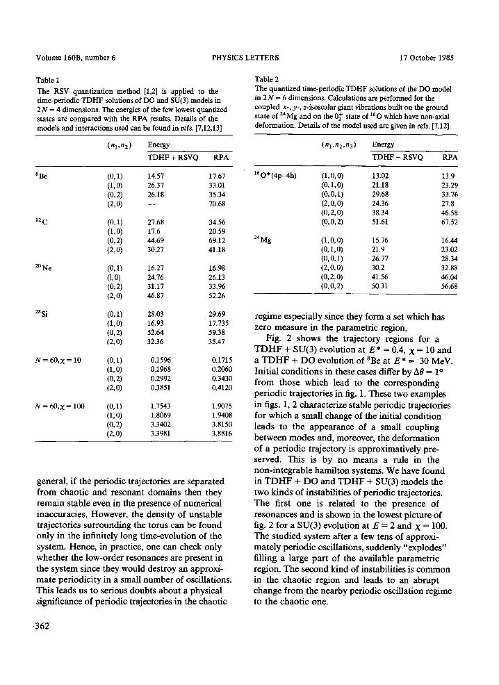
Table 1 The RSV quantization method [1,2] is applied to the time-periodic TDHF solutions of DO and SU(3) models in 2 N = 4 dimensions. The energies of the few lowest quantized states are compared with the RPA results. Details of the models and interactions used can be found in refs. [7,12,13]

(nt,n2) Energy

TDHF + RSVQ RPA

SBe

~2 C

20 Ne

(0,1) 14.57 17.67 (1,0) 26.37 33.01 (0,2) 26.18 35.34 (2,0) - - 70.68

(0,1) 27.68 34.56 (1, 0) 17.6 20.59 (0,2) 44.69 69.12 (2,0) 30.27 41.18

(0,1) 16.27 16.98 (1,0) 24.76 26.13 (0,2) 31.17 33.96 (2,0) 46.87 52.26

Table 2 The quantized time-periodic TDHF solutions of the DO model in 2 N = 6 dimensions. Calculations are performed for the coupled x-, y-, z-isoscalar giant vibrations built on the ground state of 24Mg and on the Of state of 160 which have non-axial deformation. Details of the model used are given in refs. [7,12].

(nl,n2,n3) Energy

TDHF + RSVQ RPA

16 O * (4p-4h)

24 Mg

(1,0,0) 13.02 13.9 (0,1,0) 21.18 23.29 (0,0,1) 29.68 33.76 (2,0,0) 24.36 27.8 (0,2,0) 38.34 46.58 (0,0,2) 51.61 67.52

(1,0,0) 15.76 16.44 (0,1,0) 21.9 23.02 (0,0,1) 26.77 28.34 (2,0,0) 30.2 32.88 (0,2,0) 41.56 46.04 (0,0,2) 50.31 56.68

28 Si

N= 60,X = 10

N = 60,X = 100

(0,1) 28.03 29,69 (1,0) 16.93 17.735 (0,2) 52.64 59.38 (2,0) 32.36 35.47

(0,1) 0.1596 0.1715 (1,0) 0.1968 0.2060 (0,2) 0.2992 0.3430 (2,0) 0.3851 0.4120

(0,1) 1.7543 1.9075 (1,0) 1.8069 1.9408 (0,2) 3.3402 3.8150 (2,0) 3.3981 3.8816

general , if the per iod ic t rajectories are separa ted f rom chao t ic and resonant domains then they r e m a i n s table even in the presence of numer ica l inaccurac ies . However , the dens i ty of uns tab le t ra jec tor ies su r rounding the torus can be found on ly in the inf ini te ly long t ime-evolut ion of the system. Hence , in pract ice, one can check only whe the r the low-order resonances are present in the sys tem since they would des t roy an approxi - m a t e pe r iod ic i ty in a small number of oscil lat ions. This leads us to serious doubts abou t a physical s ignif icance of per iod ic t rajectories in the chaot ic

reg ime especia l ly since they form a set which has zero measure in the pa ramet r i c region.

Fig. 2 shows the t ra jectory regions for a T D H F + SU(3) evolut ion at E * = 0.4, X = 10 and a T D H F + D O evolut ion of aBe at E * --- 30 MeV. In i t i a l cond i t ions in these cases differ by A0 = 1 o f rom those which lead to the cor responding pe r iod i c t ra jec tor ies in fig. 1. These two examples in figs. 1, 2 character ize s table per iod ic t ra jector ies for which a smal l change of the ini t ial condi t ion leads to the appea rance of a small coupl ing be tween m o d e s and, moreover, the de fo rma t ion of a pe r iod ic t ra jec tory is approx imat ive ly pre- served. This is b y no means a rule in the non - in t eg rab l e hami l ton systems. W e have found in T D H F + D O and T D H F + SU(3) models the two k inds o f ins tabi l i t ies of per iod ic trajectories. The first one is re la ted to the presence of r e sonances a n d is shown in the lowest p ic ture of fig. 2 for a SU(3) evolut ion at E = 2 and X = 100. The s tud ied sys tem after a few tens of approx i - m a t e l y pe r iod i c oscil lat ions, suddenly "exp lodes" fill ing a large pa r t of the avai lable pa ramet r i c region. The second k ind of instabi l i t ies is c o m m o n in the chao t ic region and leads to an ab rup t change f rom the nea rby per iodic osci l la t ion regime to the chao t ic one.

.362


I n conclus ion , we have p r o p o s e d a s imple m e t h o d to f ind the per iod ic t ra jector ies in the r egu la r d o m a i n of the pa ramet r i c space for general n o n - i n t e g r a b l e hami l ton i an systems. This me thod can be a p p l i e d easily for highly d imens iona l m a n i f o l d s of t r ia l wave funct ions like in the R P A

or s imi lar real is t ic nuclear s t ructure ca lcula t ions of the low- ly ing collective states. Thus, it offers the poss ib i l i t y to invest igate the s tabi l i ty of e.g. the R P A m o d e s in a more general f rame p rov ided b y the T D H F or al ike res t r ic ted hami l ton i an p rob - lems.

T h e au tho r s are grateful for the suppor t of the Cen t r e N a t i o n a l de la Recherche Scientif ique and the D a n i s h Research Counci l which great ly fac i l i t a ted this co l labora t ion .

References

[1] E. Caurier, S. Drolcli and M. Ploszajczak, Phys. Lett. 134B (1984) 1.

[2] K.K. Karl, J.J. Griffin, P.C. Lichtner and M. Dworzecka, Nucl. Phys. A332 (1979) 109.

[3] K.K. Kan, Phys. Rev. C24 (1981) 279. [4] S. Dro'2d£, J. Okolowicz and M. Ploszajczak, Phys. Lett.

115B (1982) 161. [5] E. Caurier, S. Dro2d2 and M. Ploszajczak, Phys. Lett.

150B (1985) 1; J. De Phys. C6 (1984) 361. [6] J.R. Klauder, J. Math. Phys. 8 (1967) 2392. [7] E. Caurier, S. Dro'2d~ and M. Ploszajczak, Nucl. Phys.

A425 (1984) 233. [8] A. Einstein, Verh. Dtsch. Phys. Ges. 19 (1917) 82;

M.L. Brillouin, J. Phys. (Paris) 7 (1926) 353; J.B. Keller, Ann. Phys. (NY) 4 (1958) 180.

[9] V. Maslov, Th6orie des perturbations (Dunod, Paris, 1972).

[10] A.N. Kolmogorov, Dokl. Akad. Nauk SSSR 98 (1954) 525; N.I. Arnold, Russ. Math. Surv. 18 (1963) 9; J. Moser, Nachr. Akad. Wiss. GSttingen, Math. Phys. K1. 2 (1962) 1; J. Moser, Math. Ann. 169 (1967) 136.

[11] N.N. Nekhoroshev, Russ. Math. Surv. 32 (1977) 1. [12] E. Caurier, S. Dro2d~ and M. Ploszajczak, Nucl. Phys.

A437 (1985) 407. [13] R.D. Williams and S.E. Koonin, Nucl. Phys. A391 (1982)

72. [14] D.M. Brink and E. Boeker, Nucl. Phys. A91 (1967) 1. [15] J.P. Blaizot and H. Orland, Phys. Rev. C24 (1981) 1740.

363

Documents

Time-periodic solutions of multidimensional Hamilton systems