Embed Size (px)
Citation preview
UNIVERSITÉ DE MONTRÉAL
NEW ALGORITHM TO LOCALIZE MAGNETIC ANOMALY SOURCES
CHONG LIU
DÉPARTEMENT DES GÉNIES CIVIL, GÉOLOGIQUE ET DES MINES
ÉCOLE POLYTECHNIQUE DE MONTRÉAL
MÉMOIRE PRÉSENTÉ EN VUE DE L’OBTENTION
DU DIPLÔME DE MAÎTRISE ÈS SCIENCES APPLIQUÉES
(GÉNIE MINÉRAL)
JUIN 2014
© Chong Liu, 2014.
UNIVERSITÉ DE MONTRÉAL
ÉCOLE POLYTECHNIQUE DE MONTRÉAL
UNIVERSITÉ DU QUÉBEC EN ATIBITI-TÉMISCAMINGUE
Ce mémoire intitulé:
NEW ALGORITHM TO LOCALIZE MAGNETIC ANOMALY SOURCES
présenté par : LIU Chong
en vue de l’obtention du diplôme de : Maîtrise ès sciences appliquées
a été dûment accepté par le jury d’examen constitué de :
M. MARCOTTE Denis, Ph.D., président
Mme CHENG Li Zhen, Ph.D., membre et directeur de recherche
M. CLOUTIER Vincent, Ph.D., membre et codirecteur de recherche
M. CHOUTEAU Michel, Ph.D., membre et codirecteur de recherche
M. MARESCHAL Jean-Claude, Ph.D., membre
iii
ACKNOWLEDGEMENTS
I would like to thank Professor Li Zhen CHENG, my director, whom I am grateful for
assisting and contributing to the completion of this thesis; especially for teaching me the
fundamental theory, helping me with my research, and giving me precious time to discuss
academic problems and invaluable guidance to analyze problems. I would like to thank my co-
directors, Professor Vincent CLOUTIER at UQAT and Professor Michel CHOUTEAU at
Polytechnique Montréal, for teaching me professional and theoretical knowledge and patiently
guiding me in my research. I would also like to thank Professor Xuben WANG at ChengDu
University of Technology for giving me help and guidance in my master’s research.
I would like to thank Professor Jean-claude MARESCHAL at University of Québec in
Montréal (UQAM), having accepted to review my thesis as external member of the jury. I would
like to thank also Professor Denis MARCOTTE at Polytechnique Montréal, having been the
president of jury committee for my thesis defense.
I would like to thank my colleagues, Xueping DAI, and Nacim FOUDIL-BEY, for helping
me, providing me with advices, and to have discussed the problems corresponding to my
research.
Last, but not least, I would like to thank my family, my parents and younger brother, for
providing me with support throughout my past two years when I needed it the most.
Thank You
iv
RÉSUMÉ
L’un des défis dans l’interprétation des données du champ potentiel (magnétiques et
gravimétriques) est de déterminer la profondeur de sources différentes superposées verticalement.
Jusqu’à maintenant, il n’existe pas de méthode efficace pour les distinguer. En nous basant sur la
théorie du spectre, nous avons défini une formule mathématique pour exprimer la relation entre la
profondeur d’enfouissement de la source de l’anomalie magnétique et la longueur d’onde
maximale au spectre de puissance, puis développé une nouvelle méthode d’imagerie de
profondeur. Cette nouvelle méthode a une résolution spatiale élevée pour une répartition
horizontale des sources. Pour les corps superposés verticalement, la précision d’estimation de la
profondeur augmente lorsque le corps est enfoui profondément. Lorsqu’un petit corps recouvre
un grand corps, nous pouvons facilement les séparer par la discontinuité du spectre entre les
deux. Cependant, lorsque le plus gros corps recouvre le petit, nous ne pouvons les séparer que
s’ils sont espacés d’une distance suffisamment grande.
Nous avons ensuite analysé l'impact du bruit sur la méthode d'imagerie de profondeur. Le
bruit peut provoquer une déformation grossière au résultat de la transformée de Fourier. Comme
le NSR augmente, les composantes de DC deviennent ainsi plus évidentes.
Pour ce qui est du problème de l’équivalence des sources pour les corps 2D ou 3D, nous
avons conclu que plusieurs corps ayant une géométrie différente pourraient générer une même
anomalie, mais leur centre se situe à la même profondeur. Cette équivalence ne cause aucun
problème dans l’interprétation des données magnétiques ou gravimétriques parce que la
localisation du centre de la source est la même. Si nous tentons de simuler certains corps
équivalents qui sont plus profonds que le corps causal pour compenser l’effet d’atténuation de
l’anomalie, la valeur de susceptibilité magnétique doit être au moins huit fois plus élevée que le
corps causal dans notre exemple, ce qui est non réaliste dans la nature. Finalement, nous avons
appliqué la méthode à un cas géologique réel – la région du gisement de la mine Gallen en
Abitibi. Les résultats de l’interprétation et les 19 profils n'ont pas seulement démontré des
caractéristiques géologiques connues, mais ont aussi donné de nouvelles informations sur la
structure souterraine.

v
Mots clés: Anomalie magnétique, L'analyse spectrale, La méthode Imagerie de profondeur,
Modèle géologique tridimensionnel.
vi
ABSTRACT
One of the challenges in potential field (magnetic and gravity) data interpretation is to
determine the depth of different superimposed sources. Until now there is no effective method to
distinguish them. Based on the spectrum theory, we deduced a mathematical formula to express
the relationship between the depth of the source of the magnetic anomaly and the wave-number
of the maximum power, and then developed a depth imaging method. The method has high
spatial resolution for a horizontal distribution of sources. For vertical superimposed bodies,
higher accuracy is obtained for the estimation of their depth when the depth increases. When a
small body overlays on larger body, we can easily separate them by the discontinuity of power
spectrum at the depth; however, when the bigger body hides a small body, the top depth of the
deepest body can be clearly determined only if they are separated by a certain distance.
We then analyzed the impact of noise on the depth imaging method. The noise can cause
a gross distortion to the result of Fourier transform as the NSR increases, also the DC
components become more significant.
As regarding the problem of equivalent source, we conclude that several similar bodies
having different geometries can generate similar magnetic anomalies but they are at the same
depth. This sort of equivalence does not cause problems in the interpretation of magnetic or
gravity because the source location is the same. If we try to find some equivalent bodies that are
deeper than the causative body, to compensate for the attenuation of the magnetic anomaly the
magnetic susceptibility must be at least 8 times higher than that of the causative body in our
example, this which is not realistic in nature. Finally, we applied the method to an actual
geological case - Gallen massive sulphide deposit in Abitibi region. The depth imaging results
from the airborne magnetic data did not only show some known geological features but also gave
some new information about underground structure according to the amplitude of power
spectrum, its spacing and continuity.
Keywords: Magnetic anomaly, Spectrum analysis, Depth imaging method, 3D geological model
vii
CONDENSÉ EN FRANÇAIS
1 Introduction
Le champ magnétique terrestre est généré par des sources électriques internes
(principalement par le noyau externe de la terre et l’aimantation des roches dans la croûte) de
l’ionosphère et de la magnétosphère. Nous pouvons approximativement simuler le champ
magnétique de la terre par un aimant dipolaire (William Gilbert, 1600) qui est défini par ces
angles de déclinaison (par rapport au nord) et d’inclinaison (par rapport à l’horizon). Nous
l’appelons le champ géomagnétique qui est un champ potentiel.
L’un des défis dans l’interprétation des données du champ potentiel (magnétique et gravité)
est de déterminer la profondeur des sources superposées verticalement. Bo Holm Jacobsen (1987)
a appliqué un filtre pour séparer des formations géologiques en fonction de la profondeur.
Beaucoup d’auteurs ont utilisé le prolongement du champ potentiel vers le haut et vers le bas
pour mettre en évidence différentes caractéristiques des sources peu profondes et profondes
(Jacobsen, 1987; Trompat, et al., 2003; Gordon Cooper, 2004; Chen Long-wei, et al., 2007).
Jusqu’à présent, il n’y a pas de méthode efficace pour les distinguer.
L’objectif de notre étude est de développer un nouvel outil d’interprétation afin de séparer
les sources superposées verticalement, et aussi pour essayer de distinguer les anomalies avec des
volumes différents (taille du corps géologique) et des niveaux de magnétisations différents
(nature du corps de l’anomalie causal).
Ce mémoire comporte quatre parties :
1. L'introduction présente la problématique, les objectifs de l’étude et une revue des travaux
antérieurs.
2. La deuxième partie est le noyau de ce mémoire. Après un résumé de la théorie
fondamentale sur la méthode magnétique et l’analyse du spectre, nous avons décrit, étape
par étape, la dérivation d’une nouvelle méthode de l’imagerie profonde (Depth imaging).
Par une série de tests sur les données synthétiques, nous avons validé cette méthode. Nous
avons aussi discuté en détail de l’impact des bruits sur la qualité d’interprétation et de
« l’ambiguïté » dans le résultat d’interprétation.
viii
3. Dans la troisième partie du mémoire, nous avons appliqué la méthode de l’imagerie
profonde à l’étude de la structure du dépôt de la mine Gallen. En nous basant sur les
résultats d’interprétation des 19 profils, nous avons proposé un modèle complexe
tridimensionnel pour le dépôt de la mine Gallen et des zones adjacentes.
4. La conclusion permet de faire le point sur les résultats les plus significatifs des travaux
réalisés dans le cadre de ce mémoire et des pistes de recherche possibles pour le futur.
ix
2 DÉVELOPPEMENT DE LA MÉTHODE DE L’IMAGERIE
PROFONDE SUR LA BASE DE L’ANALYSE DU SPECTRE
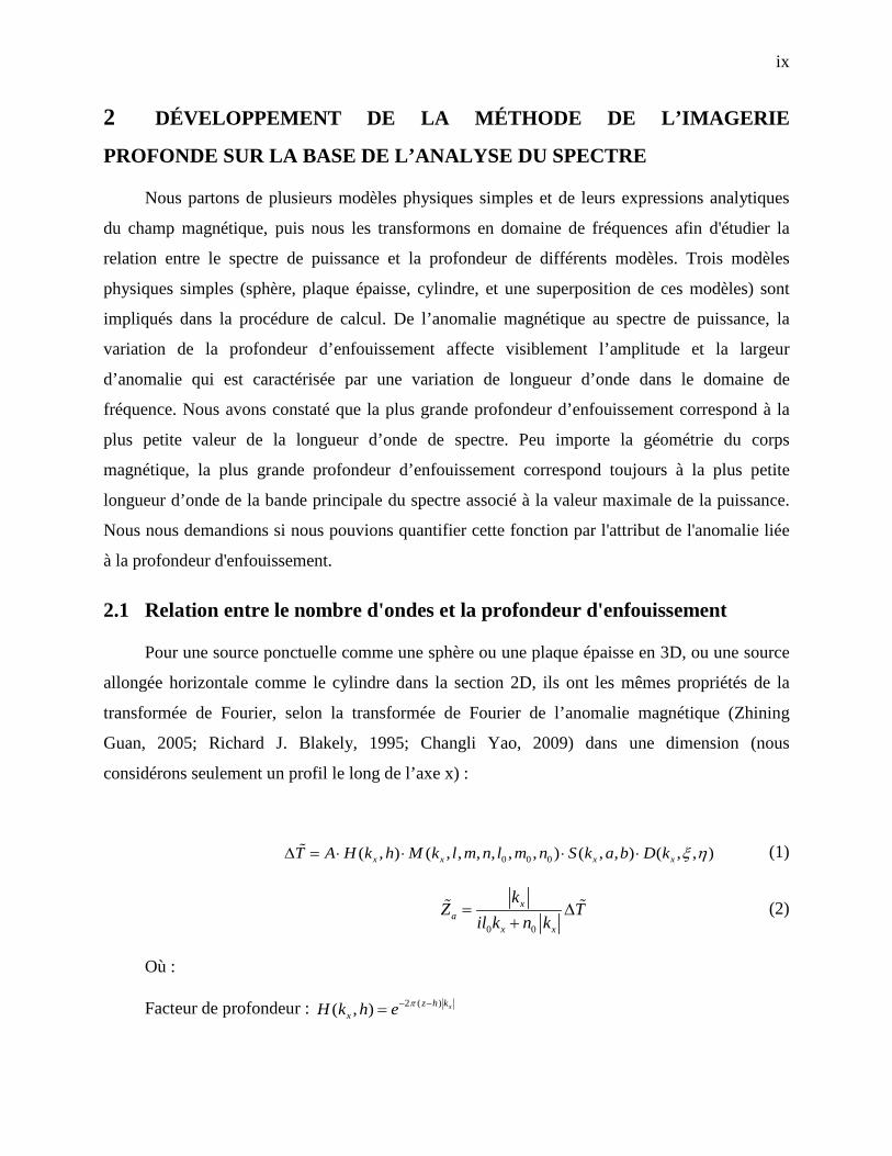
Nous partons de plusieurs modèles physiques simples et de leurs expressions analytiques
du champ magnétique, puis nous les transformons en domaine de fréquences afin d'étudier la
relation entre le spectre de puissance et la profondeur de différents modèles. Trois modèles
physiques simples (sphère, plaque épaisse, cylindre, et une superposition de ces modèles) sont
impliqués dans la procédure de calcul. De l’anomalie magnétique au spectre de puissance, la
variation de la profondeur d’enfouissement affecte visiblement l’amplitude et la largeur
d’anomalie qui est caractérisée par une variation de longueur d’onde dans le domaine de
fréquence. Nous avons constaté que la plus grande profondeur d’enfouissement correspond à la
plus petite valeur de la longueur d’onde de spectre. Peu importe la géométrie du corps
magnétique, la plus grande profondeur d’enfouissement correspond toujours à la plus petite
longueur d’onde de la bande principale du spectre associé à la valeur maximale de la puissance.
Nous nous demandions si nous pouvions quantifier cette fonction par l'attribut de l'anomalie liée
à la profondeur d'enfouissement.
2.1 Relation entre le nombre d'ondes et la profondeur d'enfouissement
Pour une source ponctuelle comme une sphère ou une plaque épaisse en 3D, ou une source
allongée horizontale comme le cylindre dans la section 2D, ils ont les mêmes propriétés de la
transformée de Fourier, selon la transformée de Fourier de l’anomalie magnétique (Zhining
Guan, 2005; Richard J. Blakely, 1995; Changli Yao, 2009) dans une dimension (nous
considérons seulement un profil le long de l’axe x) :
0 0 0( , ) ( , , , , , , ) ( , , ) ( , , )x x x xT A H k h M k l m n l m n S k a b D k ξ η∆ = ⋅ ⋅ ⋅ ⋅ (1)
0 0
xa
x x
kZ T
il k n k= ∆
+ (2)
Où :
Facteur de profondeur : 2 ( )( , ) xz h kxH k h e π− −=
x
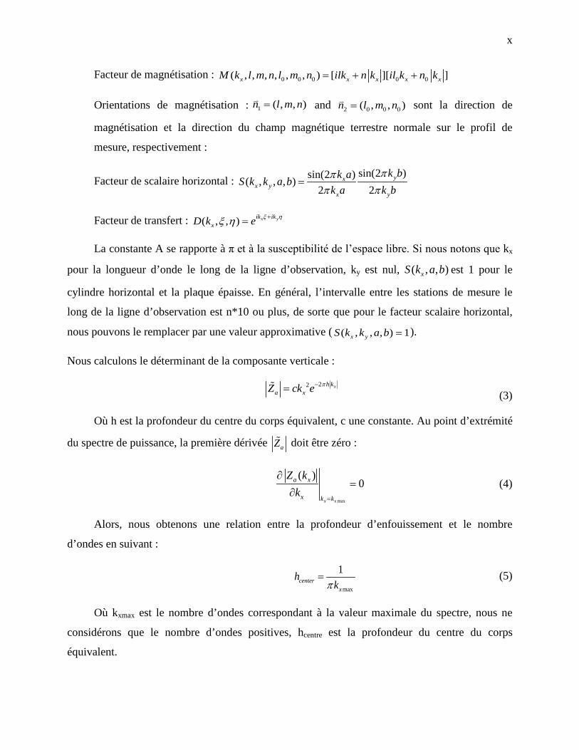
Facteur de magnétisation : 0 0 0 0 0( , , , , , , ) [ ][ ]x x x x xM k l m n l m n ilk n k il k n k= + +
Orientations de magnétisation : 1 ( , , )n l m n= and 2 0 0 0( , , )n l m n= sont la direction de
magnétisation et la direction du champ magnétique terrestre normale sur le profil de
mesure, respectivement :
Facteur de scalaire horizontal : sin(2 )sin(2 )( , , , )
2 2yx
x yx y
k bk aS k k a bk a k b
πππ π
=
Facteur de transfert : ( , , ) x yik ikxD k e ξ ηξ η +=
La constante A se rapporte à π et à la susceptibilité de l’espace libre. Si nous notons que kx
pour la longueur d’onde le long de la ligne d’observation, ky est nul, ( , , )xS k a b est 1 pour le
cylindre horizontal et la plaque épaisse. En général, l’intervalle entre les stations de mesure le
long de la ligne d’observation est n*10 ou plus, de sorte que pour le facteur scalaire horizontal,
nous pouvons le remplacer par une valeur approximative ( ( , , , ) 1x yS k k a b = ).
Nous calculons le déterminant de la composante verticale :
22 xh ka xZ ck e π−=
(3)
Où h est la profondeur du centre du corps équivalent, c une constante. Au point d’extrémité
du spectre de puissance, la première dérivée aZ doit être zéro :
max
( )0
x x
a x
x k k
Z kk
=
∂=
∂ (4)
Alors, nous obtenons une relation entre la profondeur d’enfouissement et le nombre
d’ondes en suivant :
max
1center
x
hkπ
= (5)
Où kxmax est le nombre d’ondes correspondant à la valeur maximale du spectre, nous ne
considérons que le nombre d’ondes positives, hcentre est la profondeur du centre du corps
équivalent.
xi
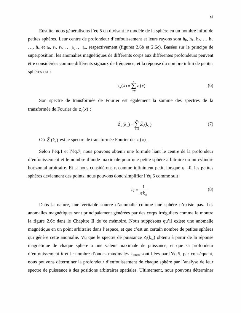
Ensuite, nous généralisons l’eq.5 en divisant le modèle de la sphère en un nombre infini de
petites sphères. Leur centre de profondeur d’enfouissement et leurs rayons sont h0, h1, h2, … hi,
…, hn et r0, r1, r2, … ri, … rn, respectivement (figures 2.6b et 2.6c). Basées sur le principe de
superposition, les anomalies magnétiques de différents corps aux différentes profondeurs peuvent
être considérées comme différents signaux de fréquence; et la réponse du nombre infini de petites
sphères est :
0( ) ( )
n
a ii
z x z x=
=∑ (6)
Son spectre de transformée de Fourier est également la somme des spectres de la
transformée de Fourier de ( )iz x :
0( ) ( )
n
a x i xi
Z k Z k=
=∑ (7)
Où ( )i xZ k est le spectre de transformée Fourier de ( )iz x .
Selon l’éq.1 et l’éq.7, nous pouvons obtenir une formule liant le centre de la profondeur
d’enfouissement et le nombre d’onde maximale pour une petite sphère arbitraire ou un cylindre
horizontal arbitraire. Et si nous considérons ri comme infiniment petit, lorsque ri→0, les petites
sphères deviennent des points, nous pouvons donc simplifier l’éq.6 comme suit :
1i
xi
hkπ
= (8)
Dans la nature, une véritable source d’anomalie comme une sphère n’existe pas. Les
anomalies magnétiques sont principalement générées par des corps irréguliers comme le montre
la figure 2.6c dans le Chapitre II de ce mémoire. Nous supposons qu’il existe une anomalie
magnétique en un point arbitraire dans l’espace, et que c’est un certain nombre de petites sphères
qui génère cette anomalie. Vu que le spectre de puissance Zi(kxi) obtenu à partir de la réponse
magnétique de chaque sphère a une valeur maximale de puissance, et que sa profondeur
d’enfouissement h et le nombre d’ondes maximales kxmax sont liées par l’éq.5, par conséquent,
nous pouvons déterminer la profondeur d’enfouissement de chaque sphère par l’analyse de leur
spectre de puissance à des positions arbitraires spatiales. Ultimement, nous pouvons déterminer
xii
une distribution de la source des anomalies magnétiques. Nous appelons cette dernière Imagerie
de profondeur.
Nous avons généré les anomalies de 14 petites sphères et ensuite utilisé l’eq.8 pour estimer
leur profondeur d’enfouissement. Les résultats sont présentés au tableau 2.2 dans le Chapitre II
de ce mémoire. L’erreur relative moyenne de l’estimation des sources profondes et peu profondes
est de 21 %. Cependant l’erreur relative est de seulement 5 % pour les sources qui se trouvent à
une profondeur supérieure à 150 mètres. Il semble que plus la profondeur d’enfouissement de la
source augmente, plus l’erreur d’estimation diminue (figure 2.7). La méthode d’imagerie de
profondeur sera donc utile pour localiser des corps enfouis profondément.
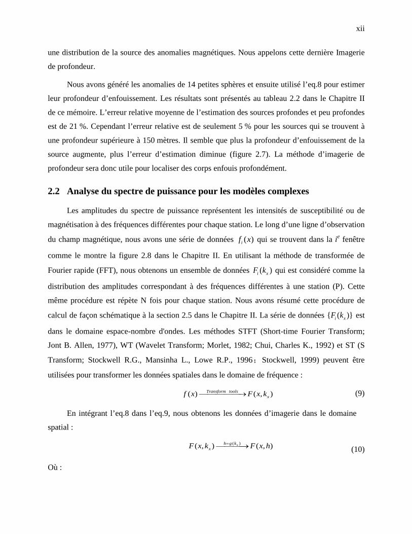
2.2 Analyse du spectre de puissance pour les modèles complexes
Les amplitudes du spectre de puissance représentent les intensités de susceptibilité ou de
magnétisation à des fréquences différentes pour chaque station. Le long d’une ligne d’observation
du champ magnétique, nous avons une série de données ( )if x qui se trouvent dans la ie fenêtre
comme le montre la figure 2.8 dans le Chapitre II. En utilisant la méthode de transformée de
Fourier rapide (FFT), nous obtenons un ensemble de données ( )i xF k qui est considéré comme la
distribution des amplitudes correspondant à des fréquences différentes à une station (P). Cette
même procédure est répète N fois pour chaque station. Nous avons résumé cette procédure de
calcul de façon schématique à la section 2.5 dans le Chapitre II. La série de données { ( )}i xF k est
dans le domaine espace-nombre d'ondes. Les méthodes STFT (Short-time Fourier Transform;
Jont B. Allen, 1977), WT (Wavelet Transform; Morlet, 1982; Chui, Charles K., 1992) et ST (S
Transform; Stockwell R.G., Mansinha L., Lowe R.P., 1996;Stockwell, 1999) peuvent être
utilisées pour transformer les données spatiales dans le domaine de fréquence :
( ) ( , )Transform toolsxf x F x k→ (9)
En intégrant l’eq.8 dans l’eq.9, nous obtenons les données d’imagerie dans le domaine
spatial :
( )( , ) ( , )xh g kxF x k F x h=→ (10)
Où :
xiii
x est la ligne d’observation;
h représente la profondeur d’enfouissement du corps causatif de l’anomalie;
xk représente la longueur d’onde ;
f(x) représente la réponse du champ magnétique (courbe noire);
fi(x) représente les données interceptées par la ie fenêtre (segment de la courbe rouge).
Nous considérons que l’amplitude (spectre de puissance) est un attribut pertinent de
l’anomalie magnétique pour chaque longueur d’onde (ou chaque profondeur) à une station. Donc,
cet attribut inclut des informations de l'intensité de la magnétisation et de la profondeur du corps
magnétique.
Nous avons appliqué la nouvelle méthode aux six modèles de sphère. Pour chaque modèle,
l’azimut de la ligne d’observation est π/2. Les sphères sont dans un champ magnétique aimanté
verticalement. Elles ont le même niveau de magnétisation et la susceptibilité est de 0.2 SI pour
chaque sphère. La force du champ magnétique incité est de 50 000 nT. Différents paramètres
géométriques sont présentés par les figures 2.32-2.37 dans le Chapitre II du mémoire.
Modèle 1 : Telles que présentées à la figure 2.32, deux sources d’anomalies sont très bien
définies par leur spectre de puissance, et leur position dans l’espace estimé par l’imagerie de
profondeur est identique à celle du modèle. La profondeur du centre de la sphère correspond à la
profondeur de la partie supérieure du spectre de puissance (partie inférieure de la figure 2.32).
Modèle 2 : Nous ajoutons une sphère plus profonde en dessous d'une des deux sphères du
modèle 1 (panneau supérieur de la figure 2.33), à la position x=0. Ces deux sphères empilées
verticalement génèrent une zone rubanée du spectre de puissance élevée (partie inférieure de la
figure 2.33). Nous ne pouvons pas distinguer les deux corps facilement, mais nous pouvons
deviner qu’il y a deux sources parce que la largeur du spectre de puissance change avec la
profondeur et parce que la zone de puissance élevée ne se ferme pas à la profondeur. L’estimation
de la position latérale de source peu profonde à l'emplacement de x=250 m correspond
exactement à la position du modèle; c’est aussi le cas pour la position latérale des deux modèles à
xiv
x=0 m. Pour la précision sur la profondeur des sphères, celle qui est enfouie à 100 mètres de
profondeur est marquée par le début de l’amincissement de spectre.
Modèles 3 et 4 : Ces modèles sont composés d’un cylindre horizontal au-dessus d'une
plaque épaisse (modèle 3), ou sous la plaque épaisse (modèle 4); ils s'étendent à l'infini le long de
l'axe y. L’inclinaison du champ magnétique est de 300 et l'azimut du profil d’observation est zéro.
Les positions du modèle et leurs paramètres géométriques sont présentés à la figure 2.34 dans le
Chapitre II. Pour le modèle 3, les emplacements du centre du cylindre sont (0, 0, -50) et (0, 0, -
150) respectivement, l'emplacement du centre de la plaque épaisse est (0, 0, -100) pour les deux
modèles.
Selon la forme du spectre habituel des sphères (centré et fermé), le spectre de puissance du
modèle 3 implique qu'il existe une autre source profonde qui a une géométrie différente de sphère
ou de cylindre. Nous pouvons voir que le haut du spectre de puissance (figure 2.34) définit très
bien la profondeur de la sphère. En plus, il y a une discontinuité de spectre qui correspond à la
profondeur du centre de la plaque épaisse, ce qui est cohérent avec les modèles 1 et 2. Nous
avons distingué ces deux corps superposés verticalement avec succès puisque la plaque épaisse a
un grand volume par rapport à la sphère. Si cette plaque épaisse se positionne au-dessus d’un
cylindre ou d’une sphère qui est caché plus profond (figure 2.35), elle pourrait engendrer une
fausse interprétation et laisser croire que la zone d’anomalie du spectre de puissance représente
un seul corps allongé verticalement (figure 2.35). Toutefois, la zone d'anomalie du spectre est
estimée entre 100 et 200 mètres de profondeur. Celle-ci récupère les deux corps et représente
toujours une interprétation raisonnable.
Modèle 5 : Comme nous ne sommes pas en mesure de distinguer le cylindre profond à
partir du prisme dans le modèle 4, nous mettons le cylindre en lieu profond (200 mètres), et nous
augmentons son rayon à 50 mètres afin d'obtenir sa réponse (figure 2.36a). L'inclinaison du
champ magnétique est de 30 degrés.
À la figure 2.36b-c, nous pouvons clairement distinguer deux zones irrégulières du spectre
de puissance. C'est définitivement prouvé que la méthode d'imagerie de profondeur peut séparer
les sources superposées verticales si elles sont à part à une certaine distance.
xv
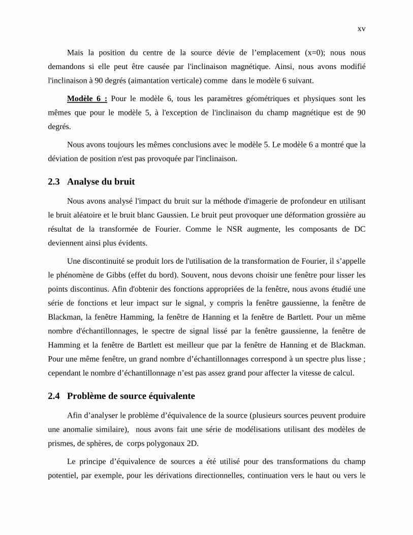
Mais la position du centre de la source dévie de l’emplacement (x=0); nous nous
demandons si elle peut être causée par l'inclinaison magnétique. Ainsi, nous avons modifié
l'inclinaison à 90 degrés (aimantation verticale) comme dans le modèle 6 suivant.
Modèle 6 : Pour le modèle 6, tous les paramètres géométriques et physiques sont les
mêmes que pour le modèle 5, à l'exception de l'inclinaison du champ magnétique est de 90
degrés.
Nous avons toujours les mêmes conclusions avec le modèle 5. Le modèle 6 a montré que la
déviation de position n'est pas provoquée par l'inclinaison.
2.3 Analyse du bruit
Nous avons analysé l'impact du bruit sur la méthode d'imagerie de profondeur en utilisant
le bruit aléatoire et le bruit blanc Gaussien. Le bruit peut provoquer une déformation grossière au
résultat de la transformée de Fourier. Comme le NSR augmente, les composants de DC
deviennent ainsi plus évidents.
Une discontinuité se produit lors de l'utilisation de la transformation de Fourier, il s’appelle
le phénomène de Gibbs (effet du bord). Souvent, nous devons choisir une fenêtre pour lisser les
points discontinus. Afin d'obtenir des fonctions appropriées de la fenêtre, nous avons étudié une
série de fonctions et leur impact sur le signal, y compris la fenêtre gaussienne, la fenêtre de
Blackman, la fenêtre Hamming, la fenêtre de Hanning et la fenêtre de Bartlett. Pour un même
nombre d'échantillonnages, le spectre de signal lissé par la fenêtre gaussienne, la fenêtre de
Hamming et la fenêtre de Bartlett est meilleur que par la fenêtre de Hanning et de Blackman.
Pour une même fenêtre, un grand nombre d’échantillonnages correspond à un spectre plus lisse ;
cependant le nombre d’échantillonnage n’est pas assez grand pour affecter la vitesse de calcul.
2.4 Problème de source équivalente
Afin d’analyser le problème d’équivalence de la source (plusieurs sources peuvent produire
une anomalie similaire), nous avons fait une série de modélisations utilisant des modèles de
prismes, de sphères, de corps polygonaux 2D.
Le principe d’équivalence de sources a été utilisé pour des transformations du champ
potentiel, par exemple, pour les dérivations directionnelles, continuation vers le haut ou vers le
xvi
bas. Nous avons discuté de ce problème en citant deux types de sources d’équivalence : source
des points confinés à une surface et des corps ayant une géométrie différente ou se situant à
différente profondeur. Selon les résultats de modélisations, nous concluons que : 1) le premier
type d’équivalence de source ne contient aucune information de la géologie; 2) plusieurs corps
ayant une géométrie différente peuvent générer une anomalie magnétique vraisemblable, mais ils
doivent se situer à la même profondeur. Cette équivalence ne pose pas de problème dans
l’interprétation des données magnétiques ou gravimétriques, car la résolution spatiale de
l’interprétation consiste à la localisation réelle de sources. En tentant de simuler certains corps
équivalents qui sont plus profonds que le corps causal, nous avons démontré que ce type de
source équivalente n’existe pas en réalité.
xvii
3 ÉTUDE DE CAS
Nous avons appliqué la méthode d'imagerie de profondeur aux données réelles recueillies à
la mine Gallen, dans la ceinture de roches vertes de l'Abitibi, au Québec.
3.1 Contexte géologique
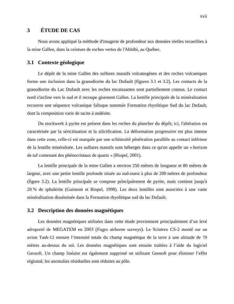
Le dépôt de la mine Gallen des sulfures massifs volcanogènes et des roches volcaniques
forme une inclusion dans la granodiorite du lac Dufault (figures 3.1 et 3.2). Les contacts de la
granodiorite du Lac Dufault avec les roches encaissantes sont partiellement connus. Le contact
nord s'incline vers le sud et il recoupe gisement Gallen. La lentille principale de la minéralisation
recouvre une séquence volcanique falisque nommée Formation rhyolitique Sud du lac Dufault,
dont la composition varie de tacite à andésite.
Du stockwerk à pyrite est présent dans les roches du plancher du dépôt; ici, l'altération est
caractérisée par la séricitisation et la silicification. La déformation progressive est plus intense
dans cette zone, celle-ci est marquée par une schistosité pénétration parallèle au contact inférieur
de la lentille minéralisée. Les sulfures massifs sont hébergés dans ce qu'on appelle un « horizon
de tuf contenant des phénocristaux de quartz » (Riopel, 2001).
La lentille principale de la mine Gallen a environ 250 mètres de longueur et 80 mètres de
largeur, avec une petite lentille profonde située au sud-ouest à plus de 200 mètres de profondeur
(figure 3.2). La lentille principale se compose principalement de pyrite, mais contient jusqu'à
20 % de sphalérite (Guimont et Riopel, 1998). Les deux lentilles sont associées à une vaste
minéralisation disséminée dans la Formation rhyolitique sud du lac Dufault.
3.2 Description des données magnétiques
Les données magnétiques utilisées dans cette étude proviennent principalement d’un levé
aéroporté de MEGATEM en 2003 (Fugro airborne surveys). Le Scintrex CS-2 monté sur un
avion Tash-12 mesure l’intensité totale du champ magnétique de la terre à une altitude de 70
mètres au-dessus du sol. Les données magnétiques sont ensuite traitées à l’aide du logiciel
Geosoft. Un champ linéaire est également supprimé en utilisant Geosoft pour éliminer l’effet
régional; les anomalies résiduelles sont réduites au pôle.
xviii
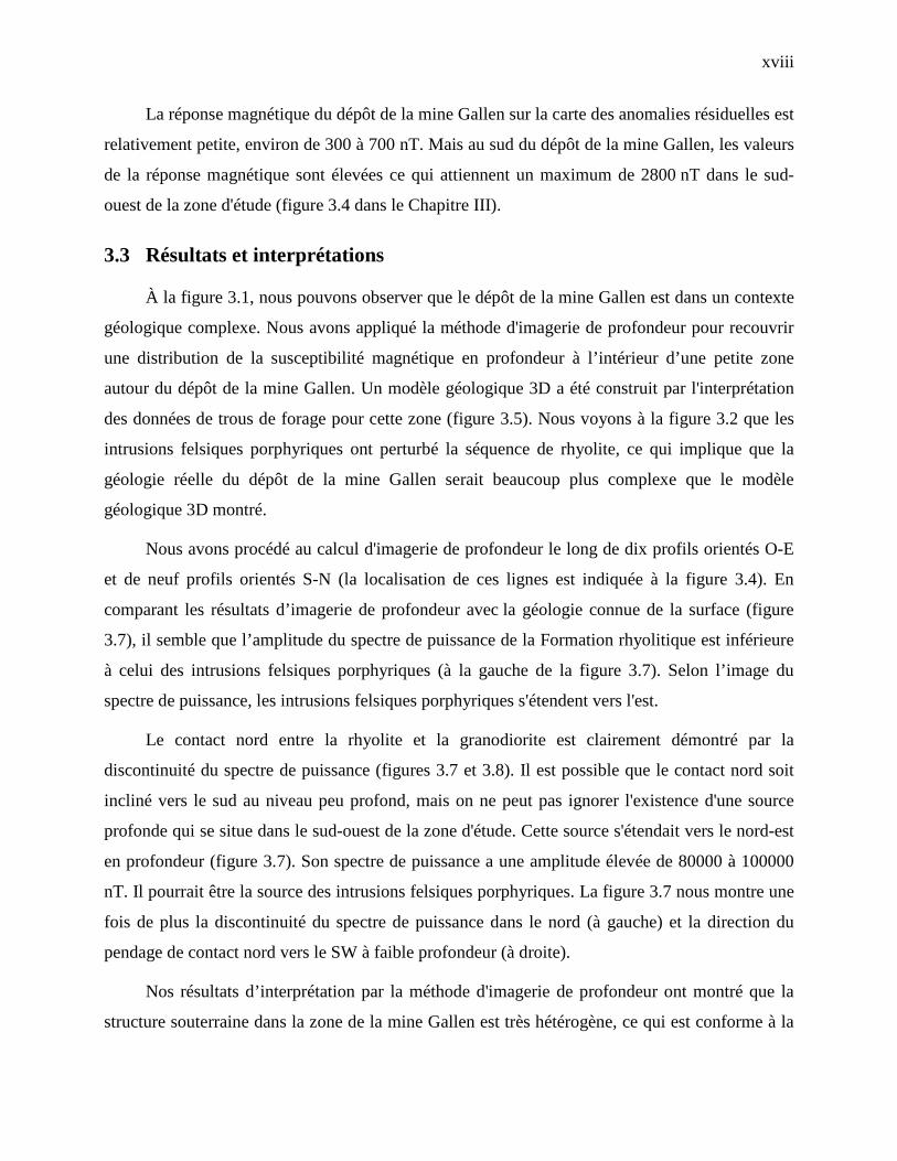
La réponse magnétique du dépôt de la mine Gallen sur la carte des anomalies résiduelles est
relativement petite, environ de 300 à 700 nT. Mais au sud du dépôt de la mine Gallen, les valeurs
de la réponse magnétique sont élevées ce qui attiennent un maximum de 2800 nT dans le sud-
ouest de la zone d'étude (figure 3.4 dans le Chapitre III).
3.3 Résultats et interprétations
À la figure 3.1, nous pouvons observer que le dépôt de la mine Gallen est dans un contexte
géologique complexe. Nous avons appliqué la méthode d'imagerie de profondeur pour recouvrir
une distribution de la susceptibilité magnétique en profondeur à l’intérieur d’une petite zone
autour du dépôt de la mine Gallen. Un modèle géologique 3D a été construit par l'interprétation
des données de trous de forage pour cette zone (figure 3.5). Nous voyons à la figure 3.2 que les
intrusions felsiques porphyriques ont perturbé la séquence de rhyolite, ce qui implique que la
géologie réelle du dépôt de la mine Gallen serait beaucoup plus complexe que le modèle
géologique 3D montré.
Nous avons procédé au calcul d'imagerie de profondeur le long de dix profils orientés O-E
et de neuf profils orientés S-N (la localisation de ces lignes est indiquée à la figure 3.4). En
comparant les résultats d’imagerie de profondeur avec la géologie connue de la surface (figure
3.7), il semble que l’amplitude du spectre de puissance de la Formation rhyolitique est inférieure
à celui des intrusions felsiques porphyriques (à la gauche de la figure 3.7). Selon l’image du
spectre de puissance, les intrusions felsiques porphyriques s'étendent vers l'est.
Le contact nord entre la rhyolite et la granodiorite est clairement démontré par la
discontinuité du spectre de puissance (figures 3.7 et 3.8). Il est possible que le contact nord soit
incliné vers le sud au niveau peu profond, mais on ne peut pas ignorer l'existence d'une source
profonde qui se situe dans le sud-ouest de la zone d'étude. Cette source s'étendait vers le nord-est
en profondeur (figure 3.7). Son spectre de puissance a une amplitude élevée de 80000 à 100000
nT. Il pourrait être la source des intrusions felsiques porphyriques. La figure 3.7 nous montre une
fois de plus la discontinuité du spectre de puissance dans le nord (à gauche) et la direction du
pendage de contact nord vers le SW à faible profondeur (à droite).
Nos résultats d’interprétation par la méthode d'imagerie de profondeur ont montré que la
structure souterraine dans la zone de la mine Gallen est très hétérogène, ce qui est conforme à la
xix
carte géologique détaillée (figure 3.2). Notre étude a proposé une nouvelle approche pour
l'interprétation des données magnétiques.
xx
4 CONCLUSIONS
Nous avons étudié les caractéristiques du spectre de puissance du champ magnétique dans
le domaine de fréquence, ce qui nous a permis de constater qu’il y a une corrélation entre la
puissance de spectre et la profondeur d'enfouissement de la source de l'anomalie. Nous avons
développé une nouvelle formule mathématique pour exprimer la relation entre la profondeur
d'enfouissement et le nombre d'ondes du spectre de puissance. Nous avons ensuite généralisé
cette formule à une situation générale et développé une nouvelle méthode d'imagerie en
profondeur pour l’interprétation des données magnétiques.
En utilisant des modèles synthétiques, nous avons testé cette nouvelle méthode. Pour les
sources horizontales, nous pouvons estimer leur profondeur et leur localisation latérale à haute
précision. Lorsque la profondeur d'enfouissement des sources augmente, nous obtenons une plus
grande précision de l'estimation par l’analyse de leur spectre de puissance. Pour les corps
superposés verticalement, nous pouvons estimer précisément la profondeur de la source peu
profonde. Si un petit corps recouvre un corps plus grand, nous pouvons facilement les séparer par
une discontinuité du spectre. Toutefois, lorsque le corps plus grand cache un petit en dessous,
nous ne pouvons les distinguer que s'ils sont suffisamment espacés.
Pour les anomalies magnétiques, le bruit peut provoquer une déformation grossière au
résultat de la transformée de Fourier comme le NSR augmente; ainsi les composants de DC
deviennent plus évidents. L’effet du bruit sur les composants avec un petit nombre d'ondes est
plus petit que ceux avec un grand nombre d'ondes pour le même rapport de signal-bruit.
À propos du problème d’équivalence de la source, selon nos études, il est possible que
plusieurs corps magnétiques à la même profondeur puissent produire une seule anomalie.
Cependant, il n’affecte que la forme du corps causal sans affecter le positionnement précis de la
source, ce qui est le plus important facteur dans l’exploration minière. Pour un empilage vertical
de plusieurs corps magnétiques, l'effet d'augmentation de la profondeur d’enfouissement sur la
forme d'anomalie est non compensable par la variation de la susceptibilité. Par conséquent, il est
donc possible de distinguer les corps à différentes profondeurs par notre nouvelle méthode.
L’effet du bord dans la transformation de Fourier (le phénomène de Gibbs) est considéré
dans notre calcul. En utilisant des fenêtres pour lisser le signal, les résultats de la transformée de
xxi
Fourier sont bien meilleurs que ceux du signal d'origine. Le principe de choisir une fenêtre est
qu’un nombre suffisant de points d’échantillonnage, en ajustant les paramètres de la fonction de
fenêtre, fait le signal original lisse de zéros.
À travers l'étude de cas de la mine Gallen, nous démontrons également que la méthode
d'imagerie de profondeur peut produire un modèle complexe sans aucune contrainte de
discrétisation du modèle. Nous allons continuer à travailler vers des situations géologiques plus
complexes. L’ajout d’informations connues, comme la contrainte dans la procédure de calcul,
permettra d'améliorer la résolution spatiale. Nous continuerons également à trouver le lien
intrinsèque entre le spectre de puissance et les propriétés physiques, comme la susceptibilité
magnétique.
xxii
TABLE OF CONTENTS
ACKNOWLEDGEMENTS .......................................................................................................... III
RÉSUMÉ ....................................................................................................................................... IV
ABSTRACT .................................................................................................................................. VI
CONDENSÉ EN FRANÇAIS .....................................................................................................VII
TABLE OF CONTENTS .......................................................................................................... XXII
LIST OF TABLES .................................................................................................................. XXIV
LIST OF FIGURES .................................................................................................................. XXV
LIST OF SYMBOLS AND ABBREVIATIONS.................................................................... XXIX
CHAPTER 1 INTRODUCTION ............................................................................................... 1
1.1 Magnetic field .................................................................................................................. 1
1.2 Methodological development and research hypotheses ................................................... 2
1.3 Objectives ......................................................................................................................... 5
CHAPTER 2 THE DEVELOPMENT OF DEPTH IMAGING METHOD BASED ON
SPECTRUM ANALYSIS ............................................................................................................... 6
2.1 Magnetic anomaly of a sphere model .............................................................................. 6
2.2 Power spectrum analysis of single or multiple spheres .................................................... 7
2.3 Magnetic anomaly of a thick prism model ..................................................................... 11
2.4 The relationship between wave-number and depth ........................................................ 13
2.5 Power spectrum analysis for complex models ............................................................... 18
2.6 Analysis of noise and the Gibbs phenomenon ............................................................... 21
2.6.1 Noise analysis ......................................................................................................... 21
2.6.2 Gibbs phenomenon and the choice of smooth window .......................................... 31
2.7 Modeling test .................................................................................................................. 36
xxiii
2.8 Problem of equivalent source ......................................................................................... 47
2.8.1 Equivalent surface or layer ..................................................................................... 47
2.8.2 Equivalent bodies ................................................................................................... 48
CHAPTER 3 CASE STUDY .................................................................................................. 54
3.1 Geology of the Gallen Volcanogenic Massive Sulfide Deposit ..................................... 54
3.2 Magnetic data description .............................................................................................. 56
3.3 Data processing results and interpretation ..................................................................... 58
CONCLUSION ............................................................................................................................. 64
REFERENCES .............................................................................................................................. 66
xxiv
LIST OF TABLES
Table 2.1: Parameters of three sets of sphere models ...................................................................... 9
Table 2.2: Estimation of the depth of 14 spheres ........................................................................... 17
Table 2.3: List of parameters of two spheres ................................................................................. 22
Table 2.4: Parameters of prism 1 - 3 .............................................................................................. 50
Table 2.5: Parameters of prism 6, sphere and 2D polygonal body ................................................ 52
Table 3.1: Magnetic susceptibilites of rocks and minerals ............................................................ 60
Table 3.2: Koenigsberger rations (Q) for some rocks .................................................................... 60
xxv
LIST OF FIGURES
Figure 2.1: Geomagnetic field elements .......................................................................................... 6
Figure 2.2: a) two sphere models; b) upper panel, magnetic anomalies of the model 1 calculated
from eq. 1 and eq. 2 on the upper panel c) and those of the model 2 on the lower panel ........ 8
Figure 2.3: vertical magnetic anomalies (left) and their Power spectrum (right) of three sets of
models. The results of Power spectrum are normalized by their own maxima. .................... 11
Figure 2.4: Elements of thick prism ............................................................................................... 12
Figure 2.5: Vertical magnetic anomalies (upward) of thick prisms and their Power spectrum at
different depths ....................................................................................................................... 13
Figure 2.6: Discretization from sphere model to an arbitrary model ............................................. 16
Figure 2.7: Correlation between depth and wave-number ............................................................. 18
Figure 2.8: Sketch of space-wavenumber-domain analysis ........................................................... 19
Figure 2.9: Complex models with three (a1) and two spheres (a2); STFT spectrum of their
magnetic anomalies (b1 and b2) ............................................................................................. 21
Figure 2.10: NSR=1%, (a) Random noise (NSR=1%), (b) original signal and the signal plus noise
and (c) spectrum of FFT of shallow sphere 1 ......................................................................... 23
Figure 2.11: NSR=3%, (a) Random noise (NSR=3%), (b) original signal and the signal plus
noise, (c) spectrum of FFT and (d) spectrum of FFT deleted DC component of shallow
sphere 1 .................................................................................................................................. 23
Figure 2.12: NSR=5%, (a) Random noise (NSR=5%), (b) original signal and the signal plus
noise, (c) spectrum of FFT and (d) spectrum of FFT deleted DC component of shallow
sphere 1 .................................................................................................................................. 24
Figure 2.13: NSR=10%, (a) Random noise (NSR=10%), (b) original signal and the signal plus
noise, (c) spectrum of FFT and (d) spectrum of FFT deleted DC component of shallow
sphere 1 .................................................................................................................................. 24
Figure 2.14: NSR=1%, (a) Random noise (NSR=1%), (b) original signal and the signal plus noise
and (c) spectrum of FFT of deep sphere 2 ............................................................................. 25
xxvi
Figure 2.15: NSR=3%, (a) Random noise (NSR=3%), (b) original signal and the signal plus
noise, (c) spectrum of FFT and of deep sphere 2 ................................................................... 25
Figure 2.16: NSR=5%, (a) Random noise (NSR=5%), (b) original signal and the signal plus
noise, (c) spectrum of FFT and (d) spectrum of FFT deleted DC component of deep sphere 2
................................................................................................................................................ 26
Figure 2.17: NSR=10%, (a) Random noise (NSR=10%), (b) original signal and the signal plus
noise, (c) spectrum of FFT and (d) spectrum of FFT deleted DC component of deep sphere 2
................................................................................................................................................ 26
Figure 2.18: NSR=1%, (a) WGN (NSR=1%), (b) original signal and the signal plus noise, (c)
spectrum of FFT of shallow sphere 1 ..................................................................................... 28
Figure 2.19: NSR=3%, (a) WGN (NSR=3%), (b) original signal and the signal plus noise, (c)
spectrum of FFT of shallow sphere 1 ..................................................................................... 28
Figure 2.20: NSR=5%, (a) WGN (NSR=5%), (b) original signal and the signal plus noise, (c)
spectrum of FFT of shallow sphere 1 ..................................................................................... 28
Figure 2.21: NSR=8%, (a) WGN (NSR=8%), (b) original signal and the signal plus noise, (c)
spectrum of FFT of shallow sphere 1 ..................................................................................... 29
Figure 2.22: NSR=1%, (a) WGN (NSR=1%), (b) original signal and the signal plus noise, (c)
spectrum of FFT of deep sphere 2 .......................................................................................... 29
Figure 2.23: NSR=3%, (a) WGN (NSR=3%),(b) original signal and the signal plus noise, (c)
spectrum of FFT of deep sphere 2 .......................................................................................... 29
Figure 2.24: NSR=5%, (a) WGN (NSR=5%), (b) original signal and the signal plus noise, (c)
spectrum of FFT of deep sphere 2 .......................................................................................... 30
Figure 2.25: NSR=8%, (a) WGN (NSR=8%), (b) original signal and the signal plus noise, (c)
spectrum of FFT of deep sphere 2 .......................................................................................... 30
Figure 2.26: Signal with a constant signal with zero frequency .................................................... 32
Figure 2.27: Analysis for the impact of Gaussian window on signal: window functions (left),
spectrum of Fourier transform about original signals and signals smoothed (right) ............. 33
xxvii
Figure 2.28: Analysis for the impact of Blackman window on signal: window functions (left),
spectrum of Fourier transform about original signals and signals smoothed (right) ............. 33
Figure 2.29: Analysis for the impact of hamming window on signal: window functions (left),
spectrum of Fourier transform about original signals and signals smoothed (right) ............. 34
Figure 2.30: Analysis for the impact of hanning window on signal: window functions (left),
spectrum of Fourier transform about original signals and signals smoothed (right) ............. 35
Figure 2.31: Analysis for the impact of Bartlett window on signal: window functions (left),
spectrum of Fourier transform about original signals and signals smoothed (right) ............. 36
Figure 2.32: Model 1 (upper), the depth imaging result (lower) .................................................... 37
Figure 2.33: Model 2 (upper) and their depth image (lowers) ....................................................... 39
Figure 2.34: Model 3 (upper) and Depth imaging (lower) for the superposition of the cylinder
over (left) or under (right) the prism, window width is 256 .................................................. 41
Figure 2.35: Model 4 (upper) and Depth imaging (lower) for the superposition of the cylinder
underneath the prism, window width is 256 .......................................................................... 43
Figure 2.36: Model 5 (left) and Depth imaging (right) processed by window function with
different width for the superposition of the cylinder and the prism ....................................... 44
Figure 2.37: Model 6 (as shown in figure 2.37a) and Depth imaging results processed by window
functions with different width for the superposition of the cylinder and the prism ............... 46
Figure 2.38: A cylinder at the depth of 250m and its equivalent-sources at different depth ......... 48
Figure 2.39: Equivalent source of prisms which have the same (or different) center depth with the
causative anomaly (Prism 1) .................................................................................................. 51
Figure 2.40: 2 dimensional (2D) polygonal body .......................................................................... 53
Figure 2.41: Responses of prism, sphere and 2D polygonal body ................................................. 53
Figure 3.1: Regional geology map of the Gallen area .................................................................... 55
Figure 3.2: Detail geological map around the Gallen deposit, overlapped by magnetic survey
lines with flight direction over the Gallen deposit (left), the geological cross-section along
line A-B .................................................................................................................................. 56
xxviii
Figure 3.3: Survey system and its configureation .......................................................................... 57
Figure 3.4: Residual magnetic anomalies over the Gallen deposit, the blue cycle indicates Gallen
ore body location, white lines represent magnetic data interpretation profiles ...................... 58
Figure 3.5: Top view of 3D model (left), the 3D geological model (right) ................................... 59
Figure 3.6: Comparisons between the depth imaging at the depth of 75 m (left), detail geological
map (middle) and 3D geological model (right) ...................................................................... 59
Figure 3.7: Two cross-sections from the depth imaging 3D model (right) and their location over
the 3D geological model (left) ............................................................................................... 61
Figure 3.8: 3D view of the depth imaging results from two cross-sections ................................... 62
Figure 3.9: Three cross-sections from the depth imging 2D model (left) and their location on the
detail geological map (right) .................................................................................................. 63
xxix
LIST OF SYMBOLS AND ABBREVIATIONS
Abbreviation or Symbol Definition
, , ,A B C D Apices of prism
'A Magnetic azimuth of profile
a , b Geometric parameters of body
c Constant
( )f x Data in spatial domain
( , )xF x k Data in space-wavenumber domain
( , )F x h Data in 2-dimensional spatial domain
FFT Fast Fourier transform
GWN White Gaussian Noise
h Burial depth of geological body
centerh Depth to the center of body
I Magnetic inclination
si Effective magnetization inclination
xk Wave number of x-axis
yk Wave number of y-axis
maxxk Wave number corresponding to the maximum value of
Power spectrum
M Total intensity of magnetization
sM Effective magnetization
xM X-axis’ component of M
yM Y-axis’ component of M
zM Z-axis’ component of M
( ( ))MAX abs S Maximum of the absolute values of signal S ,
xxx
1 ( , , )n l m n= Magnetizing direction
2 0 0 0( , , )n l m n= Direction of the normal geomagnetic field on the
Measurement profile
NSR Percent ratio of noise to signal
n Numeral
randomN Random noise distributed uniformly
0N White Gaussian noise with the variance of 1
GN White Gaussian noise with specific variances
P Power spectrum
, , ,A B C Dr r r r Distance between two points
(0,1)random Random sequence distributed in the interval [0, 1]
1 2, ,S S S Signal of magnetic response
x Survey line or x-axis
aZ Vertical magnetic anomaly component in spatial domain
aZ Vertical magnetic anomaly component in wave number
domain
2b Thickness of prism
2-D, 3-D Two dimensional, three dimensional
π Circumference ratio (PI)
0µ Magnetic permeability of free space
α The dip angle of the prism
κ Magnetic susceptibility of rocks and minerals
r Radius of sphere or cylinder
, , ,A B C Dϕ ϕ ϕ ϕ Angles between Ar , Br , Cr , Dr and the vertical line
T∆ The total magnetic anomaly field in spatial domain
T∆ The total magnetic field anomaly in wave number domain
1
CHAPTER 1 INTRODUCTION
1.1 Magnetic field
The Earth magnetic field is generated by internal electric currents (mainly by the Earth's
outer core, and the magnetization of rocks in the crust) but also from ionosphere and
magnetosphere. The Earth magnetic field can be very roughly approximated by a dipole magnet
(William Gilbert, 1600), which is defined by its angles relative to the north (declination) and
relative to the horizontal (inclination), called geomagnetic field.
In the middle of 17th century, Swedes (1640) used magnetic compasses to prospect for
magnetite in Zhalkovsky (2008). Thaln made a simple magnetometer in 1879 and the magnetic
method was then formally used for mineral exploration. In 1915, Schmidt invented the knife
edge-type magnetometer (balance), the magnetic method started to be used extensively in iron
prospecting, also for studying the geological structure. In 1936, Rogachev succeeded in inventing
the airborne magnetometer, and improved the measurement range and the efficiency of the
instrument. After the Second World War, the airborne magnetic method was widely used in
prospecting metallic deposits over extensive area. In the 20th century, in the 50’s and early 60’s,
the proton-precession magnetometer was used for marine prospecting. At the same time, the
magnetic method began to be used for the study of tectonic structures and geological mapping.
Since the strength of the magnetic field from rocks (high iron content) is small compared to
the strength of the main magnetic field of the Earth, the Spherical harmonic analysis method
(Gauss, 1838) was used to simulate Earth’s main magnetic field in order to extract structural
geology information of the crust. In 1968, the International Association of Geomagnetism and
Aeronomy (IAGA) first proposed the 1965.0 Gaussian spherical harmonic analysis models. This
model was approved in 1970 by IAGA and called the international geomagnetic reference field
model (IGRF). This model, which is regarded as the mathematical model of the main
geomagnetic field and its secular variations, consists of a set of Gaussian spherical harmonic
coefficients and annual gradient coefficients. Alldredge recreated the rectangular harmonic
analysis (RHA) in 1981, and applied RHA to surface data (1981, 1982, and 1983). Nakagawa and
Yukutake (1985) and Nakagawa et al. (1985) extended its application to the analysis of satellite
data. The RHA used a plan to approximate spherical surface; therefore the area of the model is
2
limited. In order to overcome this problem, and to use the rectangular coordinate system to
replace the spherical coordinate system, Haines (1985) designed the spherical cap harmonic
analysis (SCHA) to simulate the IGRF. Since then, the SCHA is used to provide a magnetic
reference field of Canada. Because of the secular variation of the geomagnetic field, spherical
harmonic coefficients are republished every five years, and the geomagnetic map is redrawn.
Recently, the National Geophysical Data Center (NGDC) and the British Geological Survey
developed the 2010.0 - 2015.0 World Magnetic Model (WMM). By using those models, after
subtracting the main magnetic field and correcting external sources, geophysicists use the
residual magnetic field for mineral exploration and for studying underground structures.
Magnetic exploration has many merits: the magnetometer is light and easy to handle, has
high work efficiency and low cost. The most important is that the airborne magnetic method can
measure extensive areas in a short period of time; and the measurement is not restricted by the
terrain relief, providing global magnetic field anomaly information. This method is therefore
extensively used in mineral and oil prospecting, hydrogeology, environmental sounding and for
monitoring of the movement of tectonic plates.
1.2 Methodological development and research hypotheses
The availability of magnetic data increases with time, mainly due to those collected from
airborne surveys. However, we still have limited access to efficient interpretation tools for
magnetic data. There is no clear relationship between the magnetic signal (anomaly) and the rock
types as well as the depth of the magnetic anomaly’s source, due to large variability of geology in
nature. Barton (1929), Nabighian (1962), Bhattacharya (1964), Nagy (1966), and Hjelt (1972,
1974) simulated magnetic anomalies with simple geometries such as a sphere, a cylinder and a
plate. Talwani and Ewing (1960), and Talwani (1965) proposed the numerical integration method
to simulate arbitrarily shaped bodies. These numerical methods may be cumbersome to use, yet
the body to be modeled has to be divided into a large number of thin horizontal laminas (Barnett,
1976). Parker (1973), Dorman and Lewis (1974) presented other numerical methods which are
well used in potential fields; these methods involve a series expansion in terms of the Fourier
transforms of powers being considered (Barnett). Paul (1974) developed a solution for potential
fields based on a homogenous polyhedron composed of triangular facets. Plouff (1976) used
polygonal prisms to model the potential field. Barnett (1976) developed an analytical method for
3
modeling the potential field of a homogenous, arbitrary shaped, three-dimensional body. Okabe
(1979) first proposed the 3-D vertex point method to compute the response of a potential field;
the main idea is to use polyhedral bodies composed of a set of triangles, which yields high
accuracy model. Mareschal (1985), Myoung An, et al. (1990) proposed the solution of potential
fields in the frequency domain in order to reduce the computation time. Other methods used in
simulating complex models in the spatial domain are developed, as finite element methods (Zeng
Hua Lin, 1985; Guan, Zhining, 2005; Wenxiao Zhu, Wansheng Tu, Tian you Liu, 1989) and
boundary element methods (Sigh B., 2001; Zheshi Xu, Yunju Lou, 1986). Within the finite
element method, there are three approaches: the point element method, the linear element method
and the panel method. The point element method can be used in modeling the anomalies whose
physical properties are inhomogeneous in horizontal and vertical directions. The linear element
method requires that the physical properties are change regularly along straight line. The panel
method requires that the physical properties change regularly on a surface.
The magnetic inversion methods have also made a significant progress by recovering an
underground susceptibility distribution from magnetic observations. In the 70s, the Hilbert
transformation inversion method was used in magnetic interpretation for the estimation of 2-
dimensional bodies (Moon, Ushah, 1988; Norden E. Huang, Zhaohua Wu. 2008). In the 80s, a
three-dimensional derivative computation was developed (Nabighian, 1984). Werner (1955)
proposed a deconvolution method, in which model is composed of a vertical or a dipping plate
infinitely extending downward. By solving a set of linear equations, we can estimate the
horizontal position, the depth to top, magnetic susceptibility and the magnetized direction of the
model. Hartman (1971) used this method in aeromagnetic interpretation, and Hansen (1993)
extended it to an interpretation of multiple 2-dimensional anomalies. The Compudepth inversion
method, which is based on the Fourier transform, the linear phase filtering and frequency
shifting, is used to interpret the position and depth of 2-dimensional bodies (O’Brien, 1972).
Wang and Hansen (1990) used it in the interpretation of 3-dimensional polyhedrons. Thompson
(1982) proposed the Euler deconvolution which can automatically evaluate the position of the
source and rapidly make depth estimates from large amounts of magnetic data. The theory is
based upon Euler’s homogeneity relationship. Reid et al. (1990) and Mushayandebvu et al.
(2000, 2001) developed this method and resolved the stability problem. Ugalde and Morris
(2010) used the cluster analysis technique and resolved the problem of strike and dip angle for 2-
4
and 3-dimensional bodies. The source parameter imaging (SPITM) has been presented and
developed by Thurston and Smith (1997) and by Thurston, Smith and Guillon (2002); this
method assumes either a 2-D sloping contact or a 2-D dipping thin-sheet model and is based on
the complex analytic signals.
Stochastic methods have been also widely used in the inverse calculation. In the 60s,
Backus and Gilbert proposed the Backus-Gilbert inversion method based on finding the
smoothest solution. Tarantola A. (1987) developed a set of theories and methods of probability
tomography based on optimization theories, such as the Gauss-Newton method (Chen, Kemna,
Hubbard, 2008), the non-linear conjugate gradient method (Kelbert, Egbert, Schultz, 2008) and
the Monte Carlo method (Bosch, Meza, Jimenez, Honing, 2006), resolving the divergence
problem and the stability problem. After the 90s, the simulated annealing (Rothman, 1986),
neural network (Zhining Guan, Junsheng Hou, Linping Huang et al. 1998; Ziqiang Zhu,
Guoxiang Huang, 1994) and the genetic algorithm (Berg, 1990; Smith, Scales, Fischer, 1992;
Curtis, Snieder, 1997) were presented with improved stability of the solution and speed of
convergence. Peter G. Lelièvre and Oldenburg (2006) studied the magnetic forward modeling
and the inversion of self-demagnetization effects, then designed a methodology for inverting
magnetic data for subsurface magnetization and proposed a 3D magnetic inversion with a
complicated remanence. Now, Cokriging, a stochastic inversion, which is applied to provide
quantitative descriptions of natural variables distributed in space or in time and space and
minimizes the theoretical estimation error variance by using auto- and cross-correlations of
several variables (Pejman Shamsipour, et al. 2011 and 2012).
Due to the complexity of the magnetic field caused by one or more geological bodies with
inhomogeneous magnetic susceptibilities and of irregular shapes, therefore several assumptions
have been made in the above developments, such as a) the shape of the model is regular or
simple; b) magnetization is homogeneous within the body and susceptibility is isotropic in the
causative body; and c) the remanent magnetization was not considered for most of calculations.
Although simple geological bodies are easy to simulate, complex geological conditions in
actual surveys broaden huge the gap between theoretical models and actual geology.
Furthermore, by using conventional interpretation tools, different bodies can be easily
distinguished from magnetic anomalies if they are horizontally well apart, but hardly
5
distinguishable if they are superimposed vertically. In our study, we proposed a new method in
spectrum domain, which identifies not only horizontally distributed sources, but also those
superimposed vertically.
1.3 Objectives
One of the challenges in potential field (magnetic and gravity) data interpretation is to
determine the depth of different vertical superimposed sources. Bo Holm Jacobsen (1987) applied
a filter for mapping the geology at different depth levels; many authors used the upward and
downward continuation of potential fields to enhance the signal of shallow or deep sources
(Jacobsen, 1987; Trompat, Boschetti, and Hornby, 2003; Cooper, 2004; Chen Long-wei, Zhang
Hui, and Zheng Zhi-qiang, 2007). However, until now there is no effective method to distinguish
them.
The objective of our study is to develop a new interpretation tool in order to separate deep
and shallow sources and also try to discriminate magnetic anomalies with different volumes (size
of geological body) and magnetic susceptibilities (nature of the anomaly causative body).
6
CHAPTER 2 THE DEVELOPMENT OF DEPTH IMAGING METHOD
BASED ON SPECTRUM ANALYSIS
We start from several simple physical models and their magnetic field analytic expressions,
and then transform them into frequency domain in order to study the relation between the Power
spectrum & the wave-number of spectrum and the depth of various models.
2.1 Magnetic anomaly of a sphere model
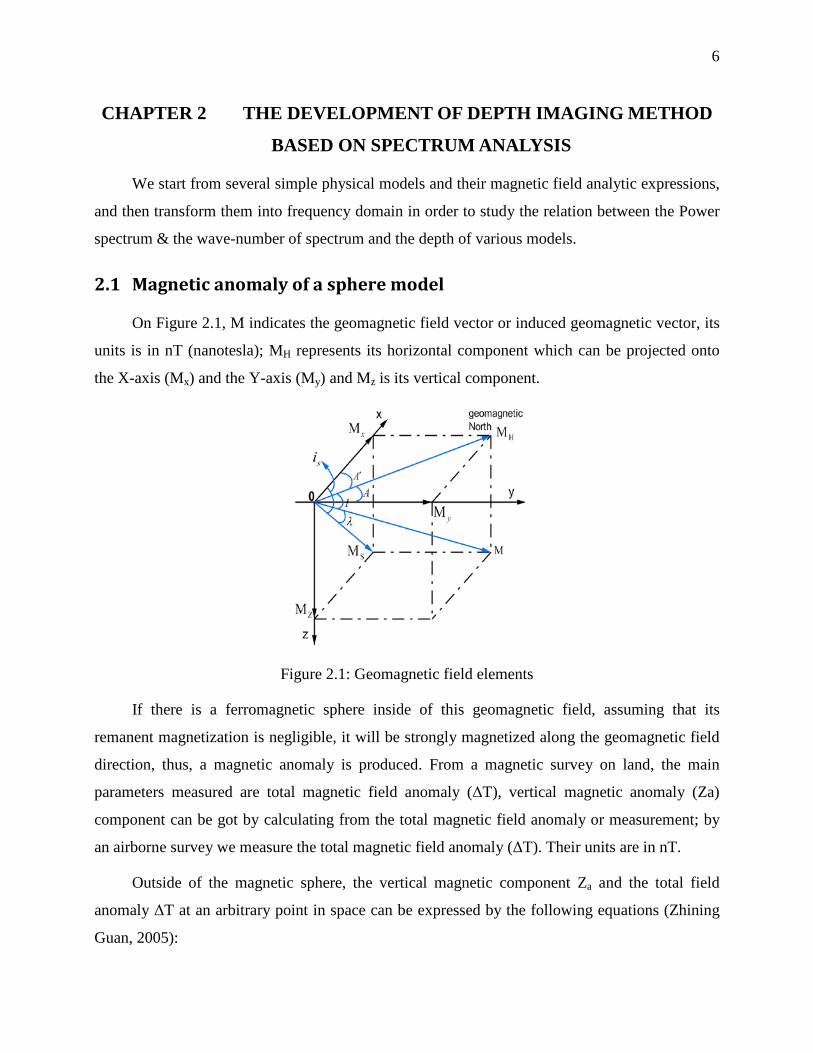
On Figure 2.1, M indicates the geomagnetic field vector or induced geomagnetic vector, its
units is in nT (nanotesla); MH represents its horizontal component which can be projected onto
the X-axis (Mx) and the Y-axis (My) and Mz is its vertical component.
Figure 2.1: Geomagnetic field elements
If there is a ferromagnetic sphere inside of this geomagnetic field, assuming that its
remanent magnetization is negligible, it will be strongly magnetized along the geomagnetic field
direction, thus, a magnetic anomaly is produced. From a magnetic survey on land, the main
parameters measured are total magnetic field anomaly (ΔT), vertical magnetic anomaly (Za)
component can be got by calculating from the total magnetic field anomaly or measurement; by
an airborne survey we measure the total magnetic field anomaly (ΔT). Their units are in nT.
Outside of the magnetic sphere, the vertical magnetic component Za and the total field
anomaly ΔT at an arbitrary point in space can be expressed by the following equations (Zhining
Guan, 2005):
7
2 2 202 2 2 5/2
' '
[(2 )sin4 ( )
3 cos cos 3 cos sin ]
amz x y h I
x y hhx I A hy I A
µπ
= − −+ +
− +
(1)
2 2 2 202 2 2 5/2
2 2 2 2 2 ' 2 2 2 2 2 '
' 2 ' '
[(2 )sin4 ( )
(2 )cos cos (2 )cos sin3 sin 2 cos 3 cos sin 2 3 sin 2 sin ]
mT h x y Ix y h
x y h I A y x h I Axh I A xy I A yh I A
µπ
∆ = − −+ +
+ − − + − −
− + −
(2)
3
0
43
m M rκ πµ
=
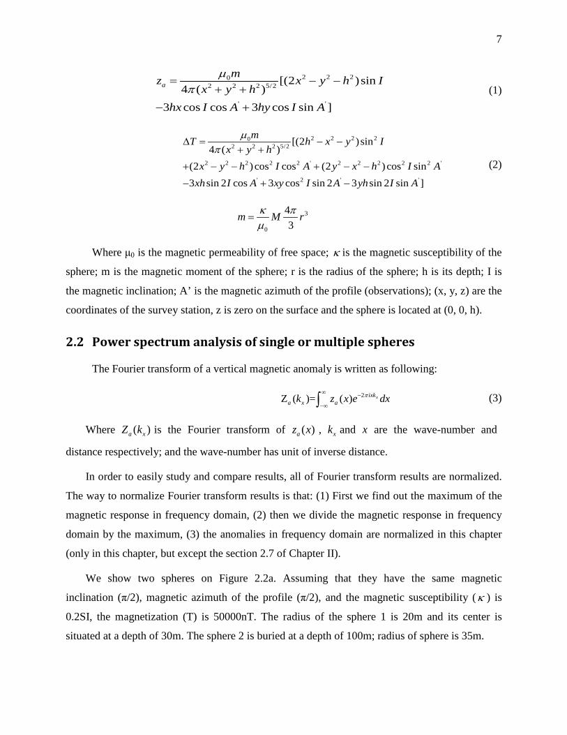
Where μ0 is the magnetic permeability of free space; κ is the magnetic susceptibility of the
sphere; m is the magnetic moment of the sphere; r is the radius of the sphere; h is its depth; I is
the magnetic inclination; A’ is the magnetic azimuth of the profile (observations); (x, y, z) are the
coordinates of the survey station, z is zero on the surface and the sphere is located at (0, 0, h).
2.2 Power spectrum analysis of single or multiple spheres
The Fourier transform of a vertical magnetic anomaly is written as following:
2Z ( )= ( ) xixka x ak z x e dxπ∞ −
−∞∫ (3)
Where ( )a xZ k is the Fourier transform of ( )az x , xk and x are the wave-number and
distance respectively; and the wave-number has unit of inverse distance.
In order to easily study and compare results, all of Fourier transform results are normalized.
The way to normalize Fourier transform results is that: (1) First we find out the maximum of the
magnetic response in frequency domain, (2) then we divide the magnetic response in frequency
domain by the maximum, (3) the anomalies in frequency domain are normalized in this chapter
(only in this chapter, but except the section 2.7 of Chapter II).
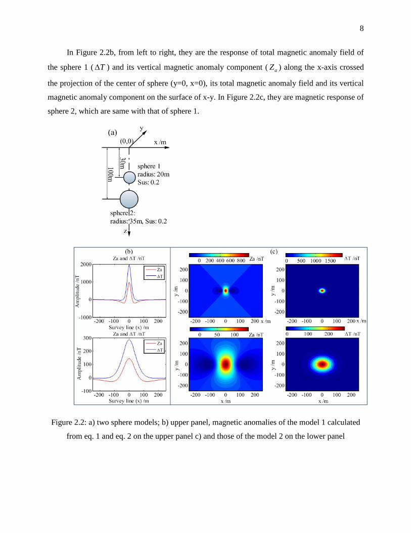
We show two spheres on Figure 2.2a. Assuming that they have the same magnetic
inclination (π/2), magnetic azimuth of the profile (π/2), and the magnetic susceptibility (κ ) is
0.2SI, the magnetization (T) is 50000nT. The radius of the sphere 1 is 20m and its center is
situated at a depth of 30m. The sphere 2 is buried at a depth of 100m; radius of sphere is 35m.
8
In Figure 2.2b, from left to right, they are the response of total magnetic anomaly field of
the sphere 1 ( T∆ ) and its vertical magnetic anomaly component ( aZ ) along the x-axis crossed
the projection of the center of sphere (y=0, x=0), its total magnetic anomaly field and its vertical
magnetic anomaly component on the surface of x-y. In Figure 2.2c, they are magnetic response of
sphere 2, which are same with that of sphere 1.
Figure 2.2: a) two sphere models; b) upper panel, magnetic anomalies of the model 1 calculated
from eq. 1 and eq. 2 on the upper panel c) and those of the model 2 on the lower panel
9
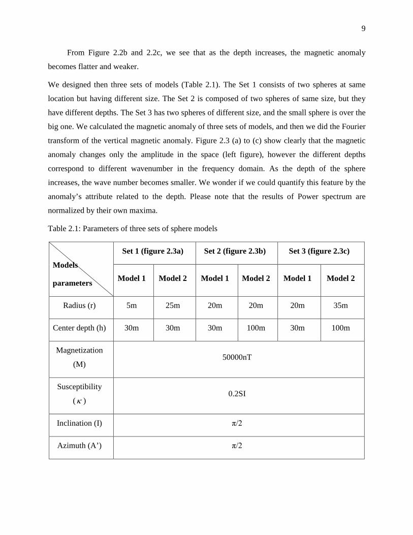
From Figure 2.2b and 2.2c, we see that as the depth increases, the magnetic anomaly
becomes flatter and weaker.
We designed then three sets of models (Table 2.1). The Set 1 consists of two spheres at same
location but having different size. The Set 2 is composed of two spheres of same size, but they
have different depths. The Set 3 has two spheres of different size, and the small sphere is over the
big one. We calculated the magnetic anomaly of three sets of models, and then we did the Fourier
transform of the vertical magnetic anomaly. Figure 2.3 (a) to (c) show clearly that the magnetic
anomaly changes only the amplitude in the space (left figure), however the different depths
correspond to different wavenumber in the frequency domain. As the depth of the sphere
increases, the wave number becomes smaller. We wonder if we could quantify this feature by the
anomaly’s attribute related to the depth. Please note that the results of Power spectrum are
normalized by their own maxima.
Table 2.1: Parameters of three sets of sphere models
Models
parameters
Set 1 (figure 2.3a) Set 2 (figure 2.3b) Set 3 (figure 2.3c)
Model 1 Model 2 Model 1 Model 2 Model 1 Model 2
Radius (r) 5m 25m 20m 20m 20m 35m
Center depth (h) 30m 30m 30m 100m 30m 100m
Magnetization
(M) 50000nT
Susceptibility
(κ ) 0.2SI
Inclination (I) π/2
Azimuth (A’) π/2
10
-1000 -800 -600 -400 -200 0 200 400 600 800 1000-500
0
500
1000
1500
2000A
mpl
itude
/nT
survey line /m
Za of model 1Za of model 2
0 0.01 0.02 0.03 0.04 0.05 0.06
0.1
0.2
0.3
0.4
0.5
0.6
0.7
0.8
0.9
1
wavenumber (1/m)
pow
er sp
ectru
m
Model 2, radius is 25m,buried depth is 30m,and other parameters of model 2 are the same as model 1
Model 1, radius is 5m,buried depth is 30m
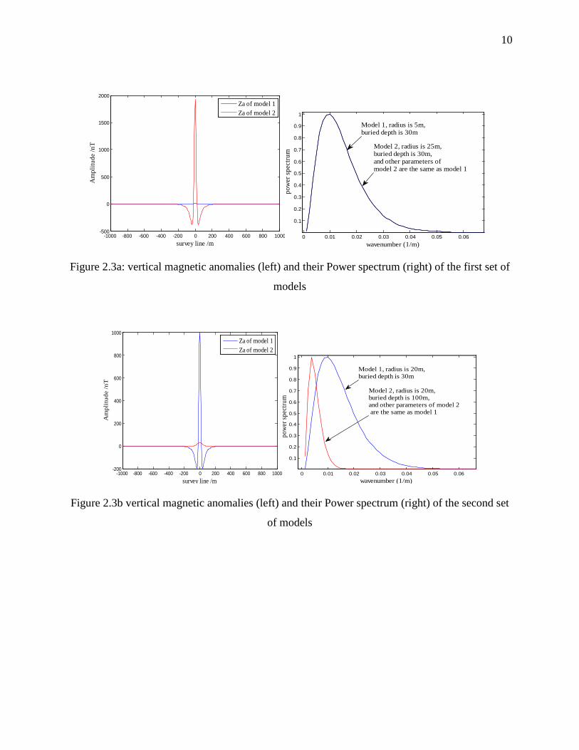
Figure 2.3a: vertical magnetic anomalies (left) and their Power spectrum (right) of the first set of
models
-1000 -800 -600 -400 -200 0 200 400 600 800 1000-200
0
200
400
600
800
1000
Am
plit
ude
/nT
survey line /m
Za of model 1Za of model 2
0 0.01 0.02 0.03 0.04 0.05 0.06
0.1
0.2
0.3
0.4
0.5
0.6
0.7
0.8
0.9
1
wavenumber (1/m)
powe
r spe
ctru
m
Model 2, radius is 20m,buried depth is 100m,and other parameters of model 2 are the same as model 1
Model 1, radius is 20m,buried depth is 30m
Figure 2.3b vertical magnetic anomalies (left) and their Power spectrum (right) of the second set
of models
11
-1000 -800 -600 -400 -200 0 200 400 600 800 1000-200
0
200
400
600
800
1000
Am
plitu
de /n
T
survey line /m
Za of model 1Za of model 2
0.01 0.02 0.03 0.04 0.05 0.06
0.1
0.2
0.3
0.4
0.5
0.6
0.7
0.8
0.9
1
wavenumber (1/m)
pow
er s
pect
rum
Model 2, radius is 35mburied depth is 100mother patameters of model 2 are the same as model1
Model 1, radius is 20mburied depth is 30m
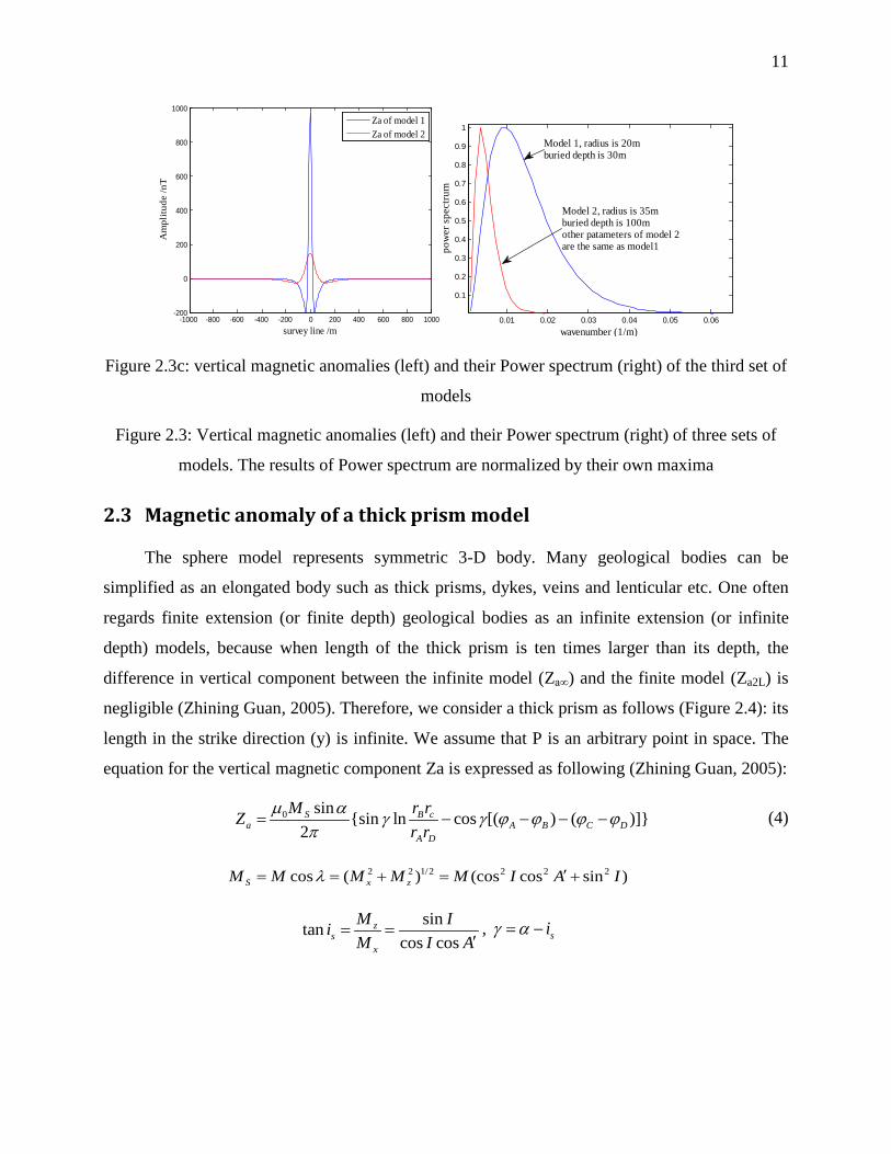
Figure 2.3c: vertical magnetic anomalies (left) and their Power spectrum (right) of the third set of
models
Figure 2.3: Vertical magnetic anomalies (left) and their Power spectrum (right) of three sets of
models. The results of Power spectrum are normalized by their own maxima
2.3 Magnetic anomaly of a thick prism model
The sphere model represents symmetric 3-D body. Many geological bodies can be
simplified as an elongated body such as thick prisms, dykes, veins and lenticular etc. One often
regards finite extension (or finite depth) geological bodies as an infinite extension (or infinite
depth) models, because when length of the thick prism is ten times larger than its depth, the
difference in vertical component between the infinite model (Za∞) and the finite model (Za2L) is
negligible (Zhining Guan, 2005). Therefore, we consider a thick prism as follows (Figure 2.4): its
length in the strike direction (y) is infinite. We assume that P is an arbitrary point in space. The
equation for the vertical magnetic component Za is expressed as following (Zhining Guan, 2005):
0 sin {sin ln cos [( ) ( )]}2S B c
a A B C DA D
M r rZr r
µ α γ γ ϕ ϕ ϕ ϕπ
= − − − − (4)
2 2 1/2 2 2 2cos ( ) (cos cos sin )S x zM M M M M I A Iλ ′= = + = +
sintancos cos
zs
x
M IiM I A
= =′
, siγ α= −
12
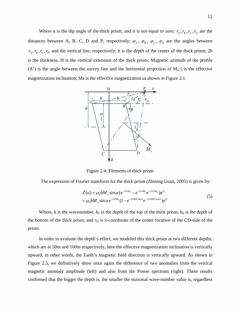
Where α is the dip angle of the thick prism, and it is not equal to zero; Ar , Br , Cr , Dr are the
distances between A, B, C, D and P, respectively; Aϕ , Bϕ , Cϕ , Dϕ are the angles between
Ar , Br , Cr , Dr and the vertical line, respectively; h is the depth of the center of the thick prism; 2b
is the thickness, H is the vertical extension of the thick prism; Magnetic azimuth of the profile
(A’) is the angle between the survey line and the horizontal projection of Ms; si is the effective
magnetization inclination; Ms is the effective magnetization as shown in Figure 2.1.
Figure 2.4: Elements of thick prism
The expression of Fourier transform for the thick prism (Zhining Guan, 2005) is given by:
1 2 2
1
2 2 20
2 2 sin 2 cos0
( ) sin ( )
sin (1 )
kh kh i kx is
kh kH i kH is
Z u bM e e e e
bM e e e e
π π π γ
π π α π α γ
µ α
µ α
− − −
− − −
= −
= − (5)
Where, k is the wavenumber, h1 is the depth of the top of the thick prism, h2 is the depth of
the bottom of the thick prism, and x2 is x-coordinate of the center location of the CD-side of the
prism.
In order to evaluate the depth’s effect, we modeled this thick prism at two different depths,
which are at 50m and 100m respectively, here the effective magnetization inclination is vertically
upward, in other words, the Earth’s magnetic field direction is vertically upward. As shown in
Figure 2.5, we definitively show once again the difference of two anomalies from the vertical
magnetic anomaly amplitude (left) and also from the Power spectrum (right). These results
confirmed that the bigger the depth is, the smaller the maximal wave-number value is, regardless
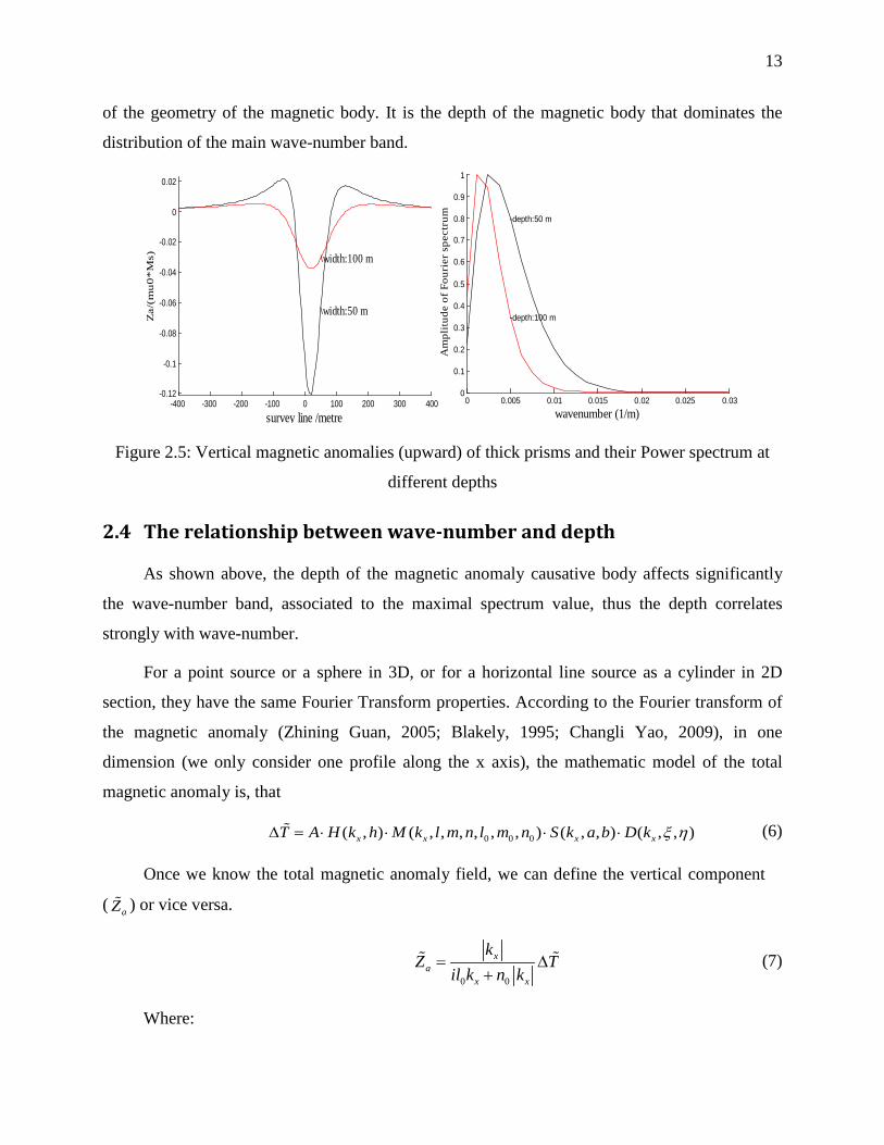
13
of the geometry of the magnetic body. It is the depth of the magnetic body that dominates the
distribution of the main wave-number band.
-400 -300 -200 -100 0 100 200 300 400-0.12
-0.1
-0.08
-0.06
-0.04
-0.02
0
0.02
\width:50 m
Za/
(mu0
*Ms)
survey line /metre
\width:100 m
0 0.005 0.01 0.015 0.02 0.025 0.030
0.1
0.2
0.3
0.4
0.5
0.6
0.7
0.8
0.9
1
-depth:50 m
Am
plit
ude
of F
ouri
er s
pect
rum
wavenumber (1/m)
-depth:100 m
Figure 2.5: Vertical magnetic anomalies (upward) of thick prisms and their Power spectrum at
different depths
2.4 The relationship between wave-number and depth
As shown above, the depth of the magnetic anomaly causative body affects significantly
the wave-number band, associated to the maximal spectrum value, thus the depth correlates
strongly with wave-number.
For a point source or a sphere in 3D, or for a horizontal line source as a cylinder in 2D
section, they have the same Fourier Transform properties. According to the Fourier transform of
the magnetic anomaly (Zhining Guan, 2005; Blakely, 1995; Changli Yao, 2009), in one
dimension (we only consider one profile along the x axis), the mathematic model of the total
magnetic anomaly is, that
0 0 0( , ) ( , , , , , , ) ( , , ) ( , , )x x x xT A H k h M k l m n l m n S k a b D k ξ η∆ = ⋅ ⋅ ⋅ ⋅ (6)
Once we know the total magnetic anomaly field, we can define the vertical component
( aZ ) or vice versa.
0 0
xa
x x
kZ T
il k n k= ∆
+ (7)
Where:
14
Depth factor: 2 ( )( , ) xz h kxH k h e π− −=
Magnetizing factor: 0 0 0 0 0( , , , , , , ) [ ][ ]x x x x xM k l m n l m n ilk n k il k n k= + +
Magnetizing orientation: 1 ( , , )n l m n= and 2 0 0 0( , , )n l m n= are the magnetizing direction
and the direction of the normal geomagnetic field on the measurement profile, respectively.
Horizontal scale factor: sin(2 )sin(2 )( , , , )
2 2yx
x yx y
k bk aS k k a bk a k b
πππ π
= , a and b are approximately
geometric parameters of an anomaly.
Shifting factor: ( , , ) x yik ikxD k e ξ ηξ η += , ( , )ξ η are the displacement in horizontal direction.
The constant A relates to π and the susceptibility of free space. If we consider wave-
number kx along the survey line (x-axis), ky is zero, thus, ( , , )xS k a b is 1 for a horizontal cylinder
and a thin prism. Also for a specific anomaly parameters a and b are constant. Therefore,
0 00 0
sin(2 )sin(2 )lim ( , , , ) lim 12 2x x
y y
yxx yk k
x yk k
k bk aS k k a bk a k b
πππ π→ →
→ →
= = (8)
We only need to calculate the items of domination for the vertical component as following.
22 xh ka xZ ck e π−= (9)
Where h is the center depth of the equivalent body and c is a constant. At the extremum of
the Power spectrum, the first derivative of aZ must be zero, that is,
max
( )0
x x
a x
xk k
Z k
k=
∂=
∂
(10)
Then we get a relation between the depth and the wave-number as follows:
max
1center
x
hkπ
= (11)
Where, maxxk is the wavenumber corresponding to the maximum spectrum value, where
only the positive wave-numbers are considered, and hcenter is the center depth of equivalent body.
15
The equation 11 represents the maximum wavenumber ( maxxk ) corresponding to the
maximum spectrum value is used. Indeed, each observed data contains near/shallow and far/deep
sources responses, which is a combination of different wavelength anomalies having different
wavenumbers. In any case, the vertical magnetic anomaly at a given point should be dominated
by sources that locate along the vertical line directly under the point of observation. We
generalize eq.11 by dividing a sphere model into an infinite number of small spheres. Their
depths and radius are h0, r0, h1, r1, h2, r2, hi, ri … hn and rn respectively (Figure 2.6b and 2.6c).
Based on the principle of superimposition, different magnetic anomalies of different sources can
be regarded as different frequency signals; and the response from an infinite number of small
spheres is given by, if we neglect demagnetization effects, then
0
0 0
( ) ( )
Z ( )= ( ) ( ) ( )x x x
n
a ii
n nixk ixk ixk
a x a i ii i
Z x Z x
k Z x e dx Z x e dx Z x e dx
=
∞ ∞ ∞− − −
−∞ −∞ −∞= =
= = =
∑
∑ ∑∫ ∫ ∫ (12)
Its Power spectrum is also the sum of the Power spectrums of ( )iz x .
0( ) ( )
n
a x i xi
Z k Z k=
=∑ (13)
Where, ( )i xZ k is the Power spectrum of ( )iZ x .
According to eq.11 and eq.13, we can obtain a formula related to the center depth and the
maximum wave-number for an arbitrary small sphere or a horizontal cylinder, that is
max
1icenter
xi
hkπ
= (14)
Our aim is to obtain a formula about the depth and the wave-number at an arbitrary point. If
we consider ri as infinitely small, that is to say ri→0, infinite small spheres become points, and
then we can get the formula about the depth and the wave-number at an arbitrary point.
1i
xi
hkπ
= (15)
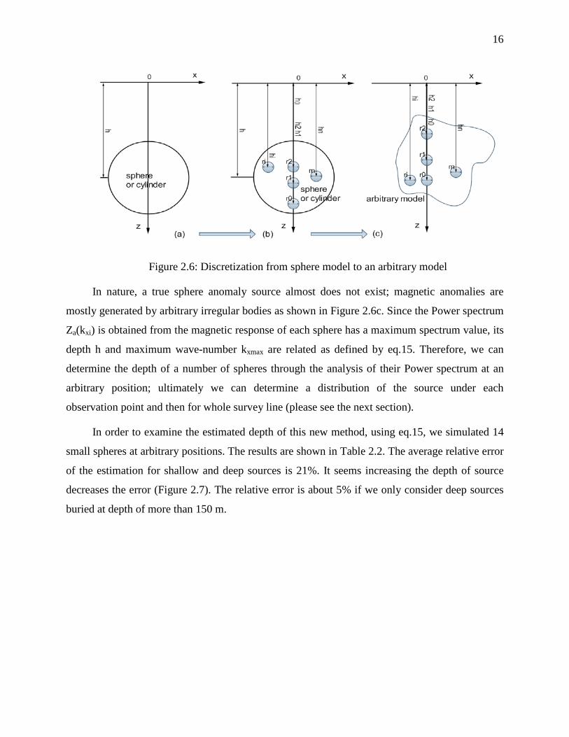
16
Figure 2.6: Discretization from sphere model to an arbitrary model
In nature, a true sphere anomaly source almost does not exist; magnetic anomalies are
mostly generated by arbitrary irregular bodies as shown in Figure 2.6c. Since the Power spectrum
Za(kxi) is obtained from the magnetic response of each sphere has a maximum spectrum value, its
depth h and maximum wave-number kxmax are related as defined by eq.15. Therefore, we can
determine the depth of a number of spheres through the analysis of their Power spectrum at an
arbitrary position; ultimately we can determine a distribution of the source under each
observation point and then for whole survey line (please see the next section).
In order to examine the estimated depth of this new method, using eq.15, we simulated 14
small spheres at arbitrary positions. The results are shown in Table 2.2. The average relative error
of the estimation for shallow and deep sources is 21%. It seems increasing the depth of source
decreases the error (Figure 2.7). The relative error is about 5% if we only consider deep sources
buried at depth of more than 150 m.
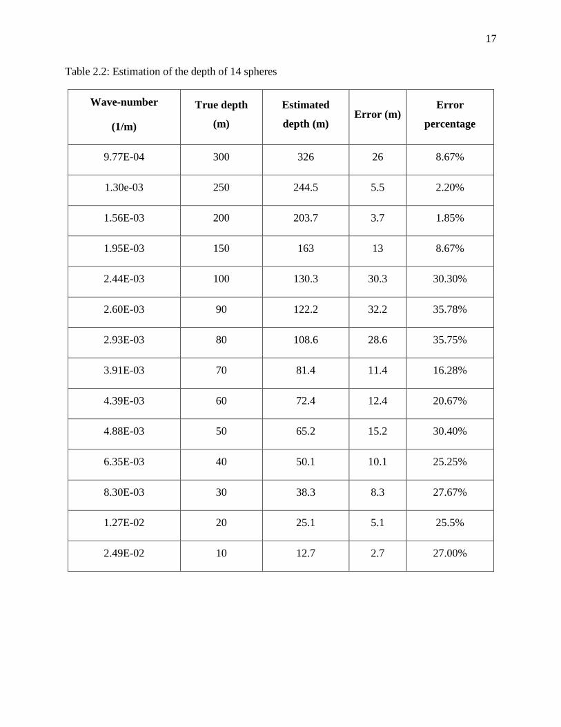
17
Table 2.2: Estimation of the depth of 14 spheres
Wave-number
(1/m)
True depth
(m)
Estimated
depth (m) Error (m)
Error
percentage
9.77E-04 300 326 26 8.67%
1.30e-03 250 244.5 5.5 2.20%
1.56E-03 200 203.7 3.7 1.85%
1.95E-03 150 163 13 8.67%
2.44E-03 100 130.3 30.3 30.30%
2.60E-03 90 122.2 32.2 35.78%
2.93E-03 80 108.6 28.6 35.75%
3.91E-03 70 81.4 11.4 16.28%
4.39E-03 60 72.4 12.4 20.67%
4.88E-03 50 65.2 15.2 30.40%
6.35E-03 40 50.1 10.1 25.25%
8.30E-03 30 38.3 8.3 27.67%
1.27E-02 20 25.1 5.1 25.5%
2.49E-02 10 12.7 2.7 27.00%
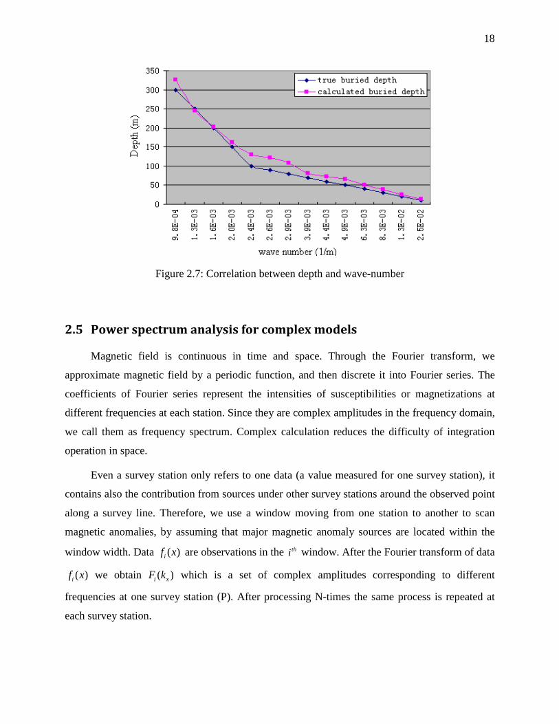
18
Figure 2.7: Correlation between depth and wave-number
2.5 Power spectrum analysis for complex models
Magnetic field is continuous in time and space. Through the Fourier transform, we
approximate magnetic field by a periodic function, and then discrete it into Fourier series. The
coefficients of Fourier series represent the intensities of susceptibilities or magnetizations at
different frequencies at each station. Since they are complex amplitudes in the frequency domain,
we call them as frequency spectrum. Complex calculation reduces the difficulty of integration
operation in space.
Even a survey station only refers to one data (a value measured for one survey station), it
contains also the contribution from sources under other survey stations around the observed point
along a survey line. Therefore, we use a window moving from one station to another to scan
magnetic anomalies, by assuming that major magnetic anomaly sources are located within the
window width. Data ( )if x are observations in the thi window. After the Fourier transform of data
( )if x we obtain ( )i xF k which is a set of complex amplitudes corresponding to different
frequencies at one survey station (P). After processing N-times the same process is repeated at
each survey station.
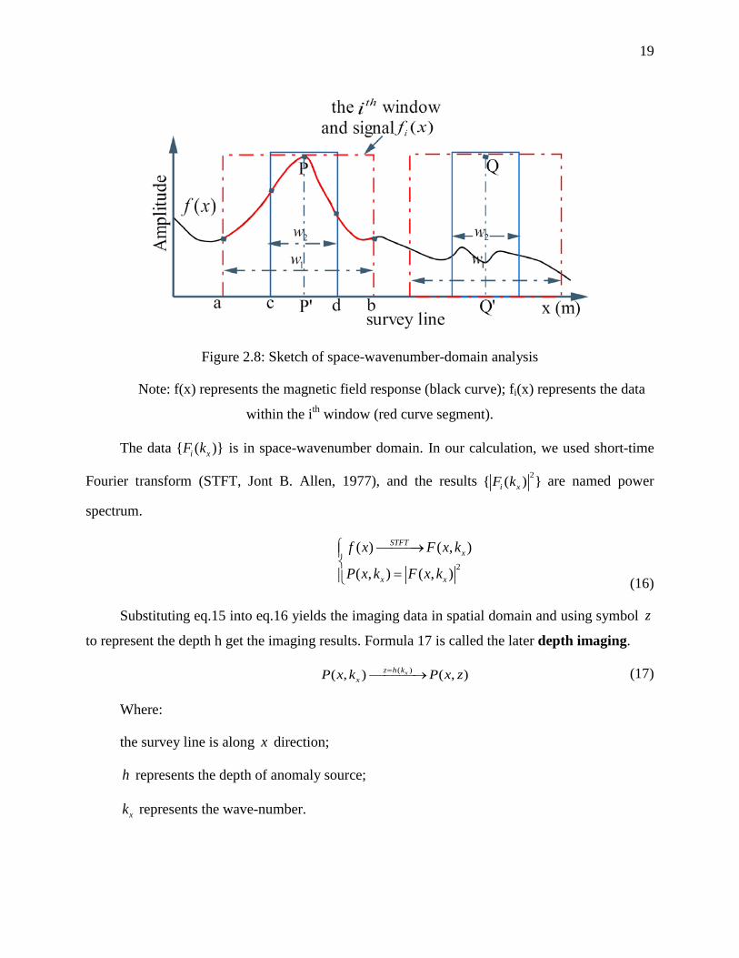
19
Figure 2.8: Sketch of space-wavenumber-domain analysis
Note: f(x) represents the magnetic field response (black curve); fi(x) represents the data
within the ith window (red curve segment).
The data { ( )}i xF k is in space-wavenumber domain. In our calculation, we used short-time
Fourier transform (STFT, Jont B. Allen, 1977), and the results 2{ ( ) }i xF k are named power
spectrum.
2
( ) ( , )
( , ) ( , )
STFTx
x x
f x F x k
P x k F x k
→
= (16)
Substituting eq.15 into eq.16 yields the imaging data in spatial domain and using symbol z
to represent the depth h get the imaging results. Formula 17 is called the later depth imaging.
( )( , ) ( , )xz h kxP x k P x z=→ (17)
Where:
the survey line is along x direction;
h represents the depth of anomaly source;
xk represents the wave-number.
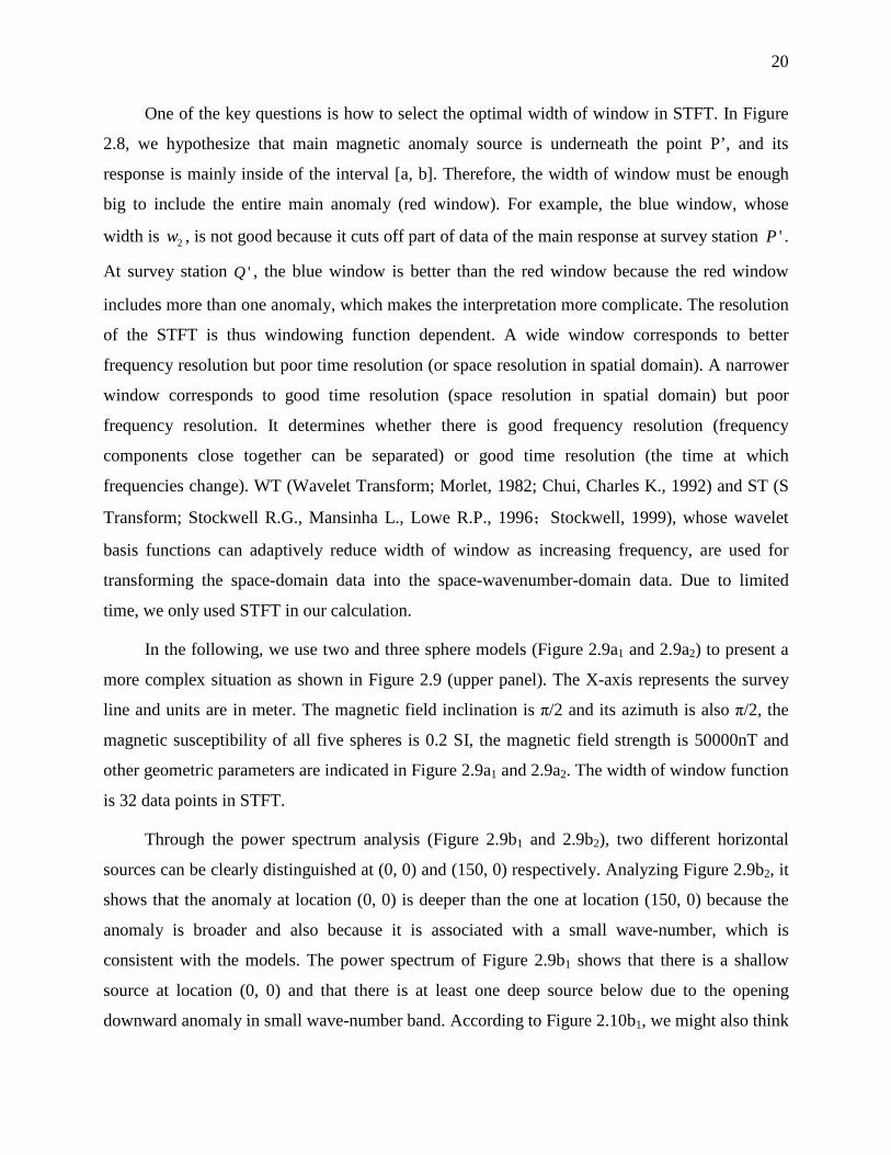
20
One of the key questions is how to select the optimal width of window in STFT. In Figure
2.8, we hypothesize that main magnetic anomaly source is underneath the point P’, and its
response is mainly inside of the interval [a, b]. Therefore, the width of window must be enough
big to include the entire main anomaly (red window). For example, the blue window, whose
width is 2w , is not good because it cuts off part of data of the main response at survey station 'P .
At survey station 'Q , the blue window is better than the red window because the red window
includes more than one anomaly, which makes the interpretation more complicate. The resolution
of the STFT is thus windowing function dependent. A wide window corresponds to better
frequency resolution but poor time resolution (or space resolution in spatial domain). A narrower
window corresponds to good time resolution (space resolution in spatial domain) but poor
frequency resolution. It determines whether there is good frequency resolution (frequency
components close together can be separated) or good time resolution (the time at which
frequencies change). WT (Wavelet Transform; Morlet, 1982; Chui, Charles K., 1992) and ST (S
Transform; Stockwell R.G., Mansinha L., Lowe R.P., 1996;Stockwell, 1999), whose wavelet
basis functions can adaptively reduce width of window as increasing frequency, are used for
transforming the space-domain data into the space-wavenumber-domain data. Due to limited
time, we only used STFT in our calculation.
In the following, we use two and three sphere models (Figure 2.9a1 and 2.9a2) to present a
more complex situation as shown in Figure 2.9 (upper panel). The X-axis represents the survey
line and units are in meter. The magnetic field inclination is π/2 and its azimuth is also π/2, the
magnetic susceptibility of all five spheres is 0.2 SI, the magnetic field strength is 50000nT and
other geometric parameters are indicated in Figure 2.9a1 and 2.9a2. The width of window function
is 32 data points in STFT.
Through the power spectrum analysis (Figure 2.9b1 and 2.9b2), two different horizontal
sources can be clearly distinguished at (0, 0) and (150, 0) respectively. Analyzing Figure 2.9b2, it
shows that the anomaly at location (0, 0) is deeper than the one at location (150, 0) because the
anomaly is broader and also because it is associated with a small wave-number, which is
consistent with the models. The power spectrum of Figure 2.9b1 shows that there is a shallow
source at location (0, 0) and that there is at least one deep source below due to the opening
downward anomaly in small wave-number band. According to Figure 2.10b1, we might also think
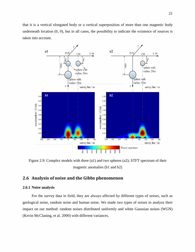
21
that it is a vertical elongated body or a vertical superposition of more than one magnetic body
underneath location (0, 0), but in all cases, the possibility to indicate the existence of sources is
taken into account.
Figure 2.9: Complex models with three (a1) and two spheres (a2); STFT spectrum of their
magnetic anomalies (b1 and b2)
2.6 Analysis of noise and the Gibbs phenomenon
2.6.1 Noise analysis
For the survey data in field, they are always affected by different types of noises, such as
geological noise, random noise and human noise. We made two types of noises to analyze their
impact on our method: random noises distributed uniformly and white Gaussian noises (WGN)
(Kevin McClaning, et al. 2000) with different variances.
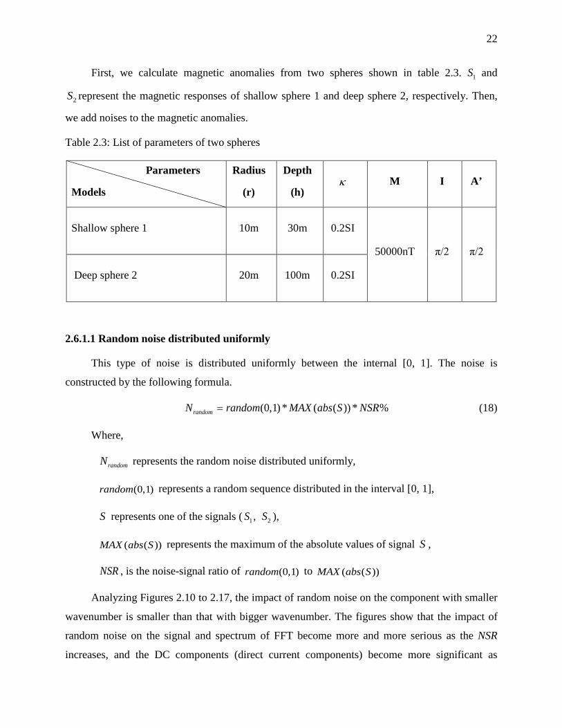
22
First, we calculate magnetic anomalies from two spheres shown in table 2.3. 1S and
2S represent the magnetic responses of shallow sphere 1 and deep sphere 2, respectively. Then,
we add noises to the magnetic anomalies.
Table 2.3: List of parameters of two spheres
Parameters
Models
Radius
(r)
Depth
(h) κ M I A’
Shallow sphere 1 10m 30m 0.2SI
50000nT π/2 π/2
Deep sphere 2 20m 100m 0.2SI
2.6.1.1 Random noise distributed uniformly
This type of noise is distributed uniformly between the internal [0, 1]. The noise is
constructed by the following formula.
(0,1) * ( ( )) * %randomN random MAX abs S NSR= (18)
Where,
randomN represents the random noise distributed uniformly,
(0,1)random represents a random sequence distributed in the interval [0, 1],
S represents one of the signals ( 1 2,S S ),
( ( ))MAX abs S represents the maximum of the absolute values of signal S ,
NSR , is the noise-signal ratio of (0,1)random to ( ( ))MAX abs S
Analyzing Figures 2.10 to 2.17, the impact of random noise on the component with smaller
wavenumber is smaller than that with bigger wavenumber. The figures show that the impact of
random noise on the signal and spectrum of FFT become more and more serious as the NSR
increases, and the DC components (direct current components) become more significant as
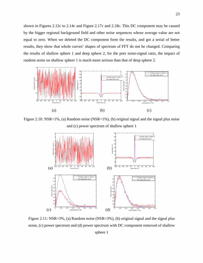
23
shown in Figures 2.12c to 2.14c and Figure 2.17c and 2.18c. This DC component may be caused
by the bigger regional background field and other noise sequences whose average value are not
equal to zero. When we deleted the DC component form the results, and got a serial of better
results, they show that whole curves’ shapes of spectrum of FFT do not be changed. Comparing
the results of shallow sphere 1 and deep sphere 2, for the peer noise-signal ratio, the impact of
random noise on shallow sphere 1 is much more serious than that of deep sphere 2.
-1000 -800 -600 -400 -200 0 200 400 600 800 10000
0.5
1
1.5
2
2.5
Am
plitu
de o
f noi
se
survey line /m-1000 -800 -600 -400 -200 0 200 400 600 800 1000
-40
-20
0
20
40
60
80
100
120
140
Am
plitu
de /n
T
survey line /m
Original signal of sphere 1the signal plus noise
0 0.01 0.02 0.03 0.04 0.05 0.06 0.070
0.1
0.2
0.3
0.4
0.5
0.6
0.7
0.8
0.9
1
Powe
r spe
ctru
m
wavenumber (1/m)
Original signal of sphere 1the signal plus noise
(a) (b) (c)
Figure 2.10: NSR=1%, (a) Random noise (NSR=1%), (b) original signal and the signal plus noise
and (c) power spectrum of shallow sphere 1
(a) -1000 -800 -600 -400 -200 0 200 400 600 800 10000
1
2
3
4
5
6
7
8
Am
plitu
de o
f noi
se
survey line /m (b) -1000 -800 -600 -400 -200 0 200 400 600 800 1000-40
-20
0
20
40
60
80
100
120
140
Am
plitu
de /n
T
survey line /m
Original signal of sphere 1the signal plus noise
(c) 0 0.01 0.02 0.03 0.04 0.05 0.06 0.070
0.1
0.2
0.3
0.4
0.5
0.6
0.7
0.8
0.9
1
Pow
er sp
ectru
m
wavenumber (1/m)
Original signal of sphere 1the signal plus noise
(d) 0 0.01 0.02 0.03 0.04 0.05 0.06 0.070
0.1
0.2
0.3
0.4
0.5
0.6
0.7
0.8
0.9
1
Pow
er sp
ectru
m
wavenumber (1/m)
Original signal of sphere 1the signal plus noise
Figure 2.11: NSR=3%, (a) Random noise (NSR=3%), (b) original signal and the signal plus
noise, (c) power spectrum and (d) power spectrum with DC component removed of shallow
sphere 1
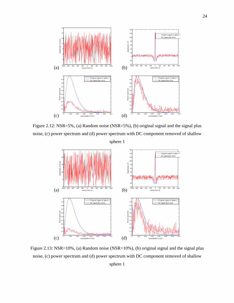
24
(a) -1000 -800 -600 -400 -200 0 200 400 600 800 10000
2
4
6
8
10
12
14
Am
plitu
de o
f noi
se
survey line /m (b) -1000 -800 -600 -400 -200 0 200 400 600 800 1000-40
-20
0
20
40
60
80
100
120
140
Am
plitu
de /n
T
survey line /m
Original signal of sphere 1the signal plus noise
(c) 0 0.01 0.02 0.03 0.04 0.05 0.06 0.070
0.1
0.2
0.3
0.4
0.5
0.6
0.7
0.8
0.9
1
Pow
er sp
ectru
m
wavenumber (1/m)
Original signal of sphere 1the signal plus noise
(d) 0 0.01 0.02 0.03 0.04 0.05 0.06 0.070
0.1
0.2
0.3
0.4
0.5
0.6
0.7
0.8
0.9
1
Pow
er sp
ectru
m
wavenumber (1/m)
Original signal of sphere 1the signal plus noise
Figure 2.12: NSR=5%, (a) Random noise (NSR=5%), (b) original signal and the signal plus
noise, (c) power spectrum and (d) power spectrum with DC component removed of shallow
sphere 1
(a) -1000 -800 -600 -400 -200 0 200 400 600 800 10000
5
10
15
20
25
Am
plitu
de o
f noi
se
survey line /m (b) -1000 -800 -600 -400 -200 0 200 400 600 800 1000-40
-20
0
20
40
60
80
100
120
140
160
Am
plitu
de /n
T
survey line /m
Original signal of sphere 1the signal plus noise
(c) 0 0.01 0.02 0.03 0.04 0.05 0.06 0.070
0.1
0.2
0.3
0.4
0.5
0.6
0.7
0.8
0.9
1
Pow
er sp
ectru
m
wavenumber (1/m)
Original signal of sphere 1the signal plus noise
(d) 0 0.01 0.02 0.03 0.04 0.05 0.06 0.070
0.1
0.2
0.3
0.4
0.5
0.6
0.7
0.8
0.9
1
Pow
er sp
ectru
m
wavenumber (1/m)
Original signal of sphere 1the signal plus noise
Figure 2.13: NSR=10%, (a) Random noise (NSR=10%), (b) original signal and the signal plus
noise, (c) power spectrum and (d) power spectrum with DC component removed of shallow
sphere 1
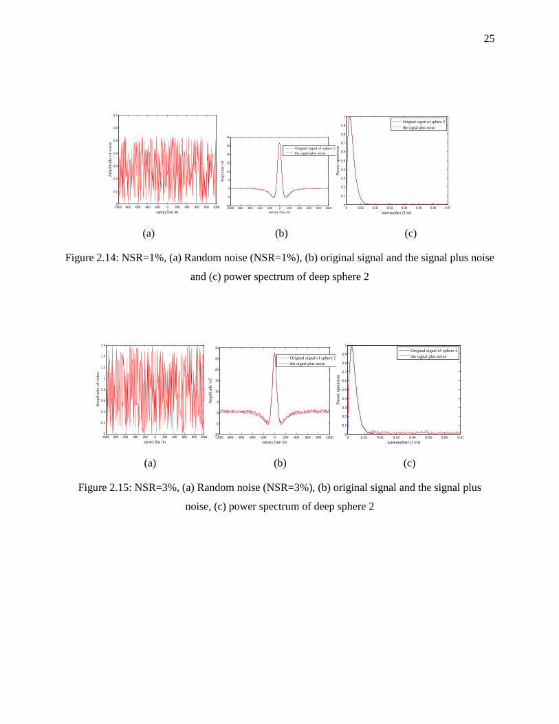
25
-1000 -800 -600 -400 -200 0 200 400 600 800 10000
0.1
0.2
0.3
0.4
0.5
0.6
0.7
Am
plit
ude
of n
oise
survey line /m-1000 -800 -600 -400 -200 0 200 400 600 800 1000
-10
-5
0
5
10
15
20
25
30
Am
plitu
de /n
T
survey line /m
Original signal of sphere 2the signal plus noise
0 0.01 0.02 0.03 0.04 0.05 0.06 0.070
0.1
0.2
0.3
0.4
0.5
0.6
0.7
0.8
0.9
1
Pow
er s
pect
rum
wavenumber (1/m)
Original signal of sphere 2the signal plus noise
(a) (b) (c)
Figure 2.14: NSR=1%, (a) Random noise (NSR=1%), (b) original signal and the signal plus noise
and (c) power spectrum of deep sphere 2
-1000 -800 -600 -400 -200 0 200 400 600 800 10000
0.2
0.4
0.6
0.8
1
1.2
1.4
1.6
Am
plit
ude
of n
oise
survey line /m-1000 -800 -600 -400 -200 0 200 400 600 800 1000
-10
-5
0
5
10
15
20
25
30
Am
plitu
de /n
T
survey line /m
Original signal of sphere 2the signal plus noise
0 0.01 0.02 0.03 0.04 0.05 0.06 0.070
0.1
0.2
0.3
0.4
0.5
0.6
0.7
0.8
0.9
1
Pow
er sp
ectru
m
wavenumber (1/m)
Original signal of sphere 2the signal plus noise
(a) (b) (c)
Figure 2.15: NSR=3%, (a) Random noise (NSR=3%), (b) original signal and the signal plus
noise, (c) power spectrum of deep sphere 2
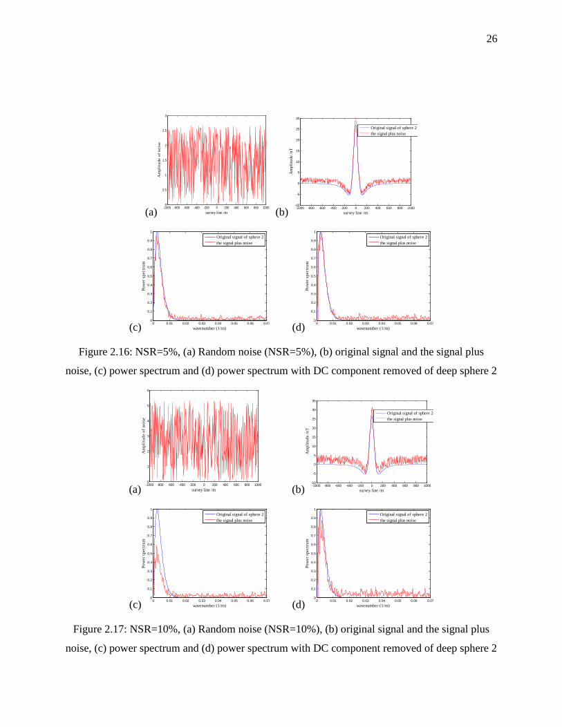
26
(a) -1000 -800 -600 -400 -200 0 200 400 600 800 10000
0.5
1
1.5
2
2.5
3
Am
plit
ude
of n
oise
survey line /m (b) -1000 -800 -600 -400 -200 0 200 400 600 800 1000-10
-5
0
5
10
15
20
25
30
Am
plitu
de /n
T
survey line /m
Original signal of sphere 2the signal plus noise
(c) 0 0.01 0.02 0.03 0.04 0.05 0.06 0.070
0.1
0.2
0.3
0.4
0.5
0.6
0.7
0.8
0.9
1
Pow
er sp
ectru
m
wavenumber (1/m)
Original signal of sphere 2the signal plus noise
(d) 0 0.01 0.02 0.03 0.04 0.05 0.06 0.070
0.1
0.2
0.3
0.4
0.5
0.6
0.7
0.8
0.9
1
Pow
er sp
ectru
m
wavenumber (1/m)
Original signal of sphere 2the signal plus noise
Figure 2.16: NSR=5%, (a) Random noise (NSR=5%), (b) original signal and the signal plus
noise, (c) power spectrum and (d) power spectrum with DC component removed of deep sphere 2
(a) -1000 -800 -600 -400 -200 0 200 400 600 800 10000
1
2
3
4
5
6
Am
plitu
de o
f noi
se
survey line /m (b) -1000 -800 -600 -400 -200 0 200 400 600 800 1000-10
-5
0
5
10
15
20
25
30
35
Am
plitu
de /n
T
survey line /m
Original signal of sphere 2the signal plus noise
(c) 0 0.01 0.02 0.03 0.04 0.05 0.06 0.070
0.1
0.2
0.3
0.4
0.5
0.6
0.7
0.8
0.9
1
Pow
er sp
ectru
m
wavenumber (1/m)
Original signal of sphere 2the signal plus noise
(d) 0 0.01 0.02 0.03 0.04 0.05 0.06 0.070
0.1
0.2
0.3
0.4
0.5
0.6
0.7
0.8
0.9
1
Pow
er sp
ectru
m
wavenumber (1/m)
Original signal of sphere 2the signal plus noise
Figure 2.17: NSR=10%, (a) Random noise (NSR=10%), (b) original signal and the signal plus
noise, (c) power spectrum and (d) power spectrum with DC component removed of deep sphere 2
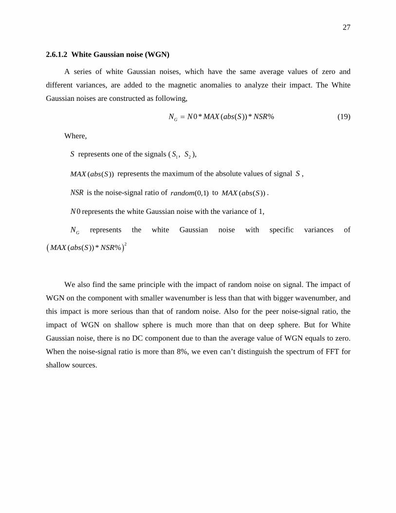
27
2.6.1.2 White Gaussian noise (WGN)
A series of white Gaussian noises, which have the same average values of zero and
different variances, are added to the magnetic anomalies to analyze their impact. The White
Gaussian noises are constructed as following,
0* ( ( )) * %GN N MAX abs S NSR= (19)
Where,
S represents one of the signals ( 1 2,S S ),
( ( ))MAX abs S represents the maximum of the absolute values of signal S ,
NSR is the noise-signal ratio of (0,1)random to ( ( ))MAX abs S .
0N represents the white Gaussian noise with the variance of 1,
GN represents the white Gaussian noise with specific variances of
( )2( ( )) * %MAX abs S NSR
We also find the same principle with the impact of random noise on signal. The impact of
WGN on the component with smaller wavenumber is less than that with bigger wavenumber, and
this impact is more serious than that of random noise. Also for the peer noise-signal ratio, the
impact of WGN on shallow sphere is much more than that on deep sphere. But for White
Gaussian noise, there is no DC component due to than the average value of WGN equals to zero.
When the noise-signal ratio is more than 8%, we even can’t distinguish the spectrum of FFT for
shallow sources.
28
-1000 -800 -600 -400 -200 0 200 400 600 800 1000-8
-6
-4
-2
0
2
4
6
8A
mpl
itude
of n
oise
survey line /m-1000 -800 -600 -400 -200 0 200 400 600 800 1000
-40
-20
0
20
40
60
80
100
120
140
Ampl
itude
/nT
survey line /m
Original signal of sphere 1the signal plus noise
0 0.01 0.02 0.03 0.04 0.05 0.06 0.070
0.1
0.2
0.3
0.4
0.5
0.6
0.7
0.8
0.9
1
Pow
er sp
ectru
m
wavenumber (1/m)
Original signal of sphere 1the signal plus noise
(a) (b) (c)
Figure 2.18: NSR=1%, (a) WGN (NSR=1%), (b) original signal and the signal plus noise, (c)
power spectrum of shallow sphere 1
-1000 -800 -600 -400 -200 0 200 400 600 800 1000-30
-25
-20
-15
-10
-5
0
5
10
15
20
Am
plitu
de o
f noi
se
survey line /m-1000 -800 -600 -400 -200 0 200 400 600 800 1000
-40
-20
0
20
40
60
80
100
120
140
Am
plitu
de /n
T
survey line /m
Original signal of sphere 1the signal plus noise
0 0.01 0.02 0.03 0.04 0.05 0.06 0.070
0.1
0.2
0.3
0.4
0.5
0.6
0.7
0.8
0.9
1
Pow
er sp
ectru
m
wavenumber (1/m)
Original signal of sphere 1the signal plus noise
(a) (b) (c)
Figure 2.19: NSR=3%, (a) WGN (NSR=3%), (b) original signal and the signal plus noise, (c)
power spectrum of shallow sphere 1
-1000 -800 -600 -400 -200 0 200 400 600 800 1000-40
-30
-20
-10
0
10
20
30
40
50
Am
plitu
de o
f noi
se
survey line /m-1000 -800 -600 -400 -200 0 200 400 600 800 1000
-60
-40
-20
0
20
40
60
80
100
120
140
Ampl
itude
/nT
survey line /m
Original signal of sphere 1the signal plus noise
0 0.01 0.02 0.03 0.04 0.05 0.06 0.070
0.1
0.2
0.3
0.4
0.5
0.6
0.7
0.8
0.9
1
Pow
er sp
ectru
m
wavenumber (1/m)
Original signal of sphere 1the signal plus noise
(a) (b) (c)
Figure 2.20: NSR=5%, (a) WGN (NSR=5%), (b) original signal and the signal plus noise, (c)
power spectrum of shallow sphere 1
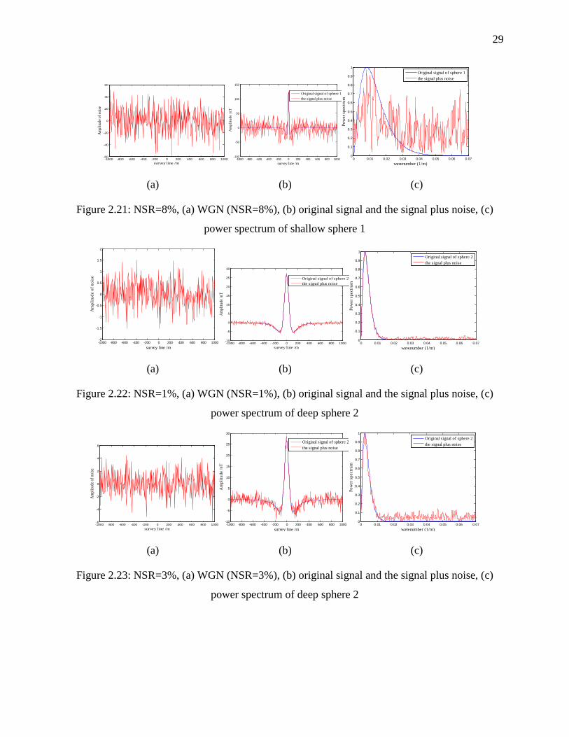
29
-1000 -800 -600 -400 -200 0 200 400 600 800 1000-60
-40
-20
0
20
40
60
Ampli
tude o
f nois
e
survey line /m-1000 -800 -600 -400 -200 0 200 400 600 800 1000
-100
-50
0
50
100
150
Am
plitu
de /n
T
survey line /m
Original signal of sphere 1the signal plus noise
0 0.01 0.02 0.03 0.04 0.05 0.06 0.070
0.1
0.2
0.3
0.4
0.5
0.6
0.7
0.8
0.9
1
Pow
er sp
ectru
m
wavenumber (1/m)
Original signal of sphere 1the signal plus noise
(a) (b) (c)
Figure 2.21: NSR=8%, (a) WGN (NSR=8%), (b) original signal and the signal plus noise, (c)
power spectrum of shallow sphere 1
-1000 -800 -600 -400 -200 0 200 400 600 800 1000-2
-1.5
-1
-0.5
0
0.5
1
1.5
2
Am
plitu
de o
f noi
se
survey line /m-1000 -800 -600 -400 -200 0 200 400 600 800 1000
-10
-5
0
5
10
15
20
25
30
Ampl
itude
/nT
survey line /m
Original signal of sphere 2the signal plus noise
0 0.01 0.02 0.03 0.04 0.05 0.06 0.070
0.1
0.2
0.3
0.4
0.5
0.6
0.7
0.8
0.9
1
Pow
er sp
ectru
mwavenumber (1/m)
Original signal of sphere 2the signal plus noise
(a) (b) (c)
Figure 2.22: NSR=1%, (a) WGN (NSR=1%), (b) original signal and the signal plus noise, (c)
power spectrum of deep sphere 2
-1000 -800 -600 -400 -200 0 200 400 600 800 1000-6
-4
-2
0
2
4
6
Ampl
itude
of no
ise
survey line /m-1000 -800 -600 -400 -200 0 200 400 600 800 1000
-10
-5
0
5
10
15
20
25
30
Am
plitu
de /n
T
survey line /m
Original signal of sphere 2the signal plus noise
0 0.01 0.02 0.03 0.04 0.05 0.06 0.070
0.1
0.2
0.3
0.4
0.5
0.6
0.7
0.8
0.9
1
Pow
er sp
ectru
m
wavenumber (1/m)
Original signal of sphere 2the signal plus noise
(a) (b) (c)
Figure 2.23: NSR=3%, (a) WGN (NSR=3%), (b) original signal and the signal plus noise, (c)
power spectrum of deep sphere 2
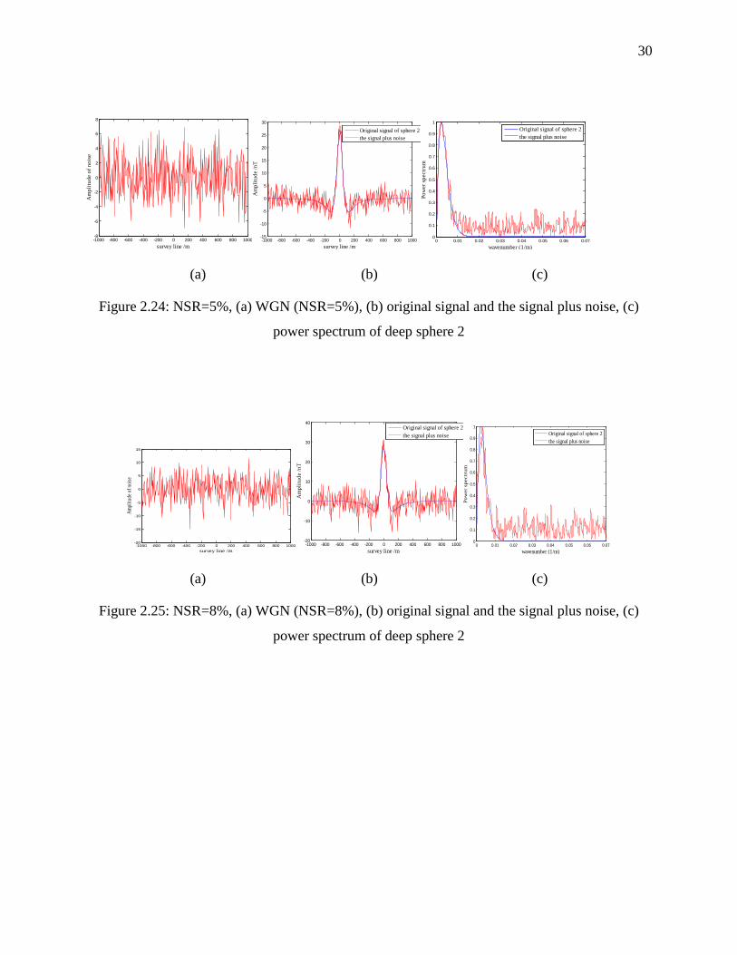
30
-1000 -800 -600 -400 -200 0 200 400 600 800 1000-8
-6
-4
-2
0
2
4
6
8
Am
plitu
de o
f noi
se
survey line /m-1000 -800 -600 -400 -200 0 200 400 600 800 1000
-15
-10
-5
0
5
10
15
20
25
30
Am
plitu
de /n
Tsurvey line /m
Original signal of sphere 2the signal plus noise
0 0.01 0.02 0.03 0.04 0.05 0.06 0.070
0.1
0.2
0.3
0.4
0.5
0.6
0.7
0.8
0.9
1
Pow
er sp
ectru
m
wavenumber (1/m)
Original signal of sphere 2the signal plus noise
(a) (b) (c)
Figure 2.24: NSR=5%, (a) WGN (NSR=5%), (b) original signal and the signal plus noise, (c)
power spectrum of deep sphere 2
-1000 -800 -600 -400 -200 0 200 400 600 800 1000-20
-15
-10
-5
0
5
10
15
Ampli
tude o
f nois
e
survey line /m-1000 -800 -600 -400 -200 0 200 400 600 800 1000
-20
-10
0
10
20
30
40
Am
plitu
de /n
T
survey line /m
Original signal of sphere 2the signal plus noise
0 0.01 0.02 0.03 0.04 0.05 0.06 0.070
0.1
0.2
0.3
0.4
0.5
0.6
0.7
0.8
0.9
1
Pow
er s
pect
rum
wavenumber (1/m)
Original signal of sphere 2the signal plus noise
(a) (b) (c)
Figure 2.25: NSR=8%, (a) WGN (NSR=8%), (b) original signal and the signal plus noise, (c)
power spectrum of deep sphere 2
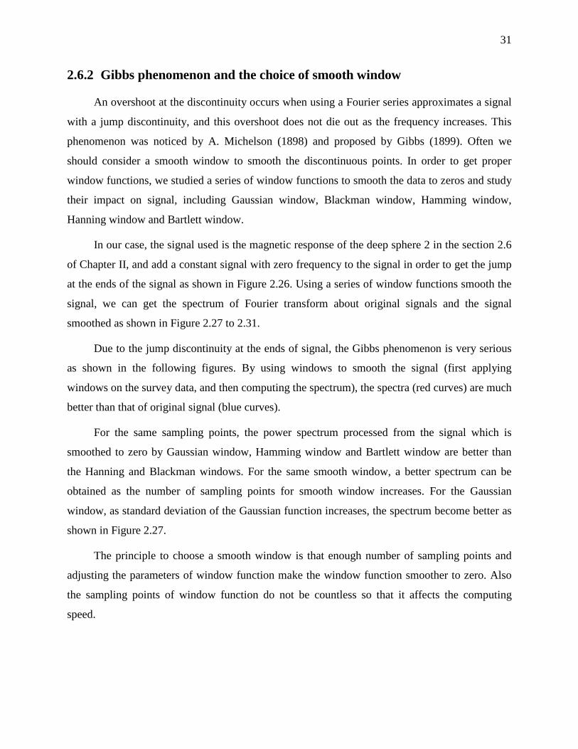
31
2.6.2 Gibbs phenomenon and the choice of smooth window
An overshoot at the discontinuity occurs when using a Fourier series approximates a signal
with a jump discontinuity, and this overshoot does not die out as the frequency increases. This
phenomenon was noticed by A. Michelson (1898) and proposed by Gibbs (1899). Often we
should consider a smooth window to smooth the discontinuous points. In order to get proper
window functions, we studied a series of window functions to smooth the data to zeros and study
their impact on signal, including Gaussian window, Blackman window, Hamming window,
Hanning window and Bartlett window.
In our case, the signal used is the magnetic response of the deep sphere 2 in the section 2.6
of Chapter II, and add a constant signal with zero frequency to the signal in order to get the jump
at the ends of the signal as shown in Figure 2.26. Using a series of window functions smooth the
signal, we can get the spectrum of Fourier transform about original signals and the signal
smoothed as shown in Figure 2.27 to 2.31.
Due to the jump discontinuity at the ends of signal, the Gibbs phenomenon is very serious
as shown in the following figures. By using windows to smooth the signal (first applying
windows on the survey data, and then computing the spectrum), the spectra (red curves) are much
better than that of original signal (blue curves).
For the same sampling points, the power spectrum processed from the signal which is
smoothed to zero by Gaussian window, Hamming window and Bartlett window are better than
the Hanning and Blackman windows. For the same smooth window, a better spectrum can be
obtained as the number of sampling points for smooth window increases. For the Gaussian
window, as standard deviation of the Gaussian function increases, the spectrum become better as
shown in Figure 2.27.
The principle to choose a smooth window is that enough number of sampling points and
adjusting the parameters of window function make the window function smoother to zero. Also
the sampling points of window function do not be countless so that it affects the computing
speed.
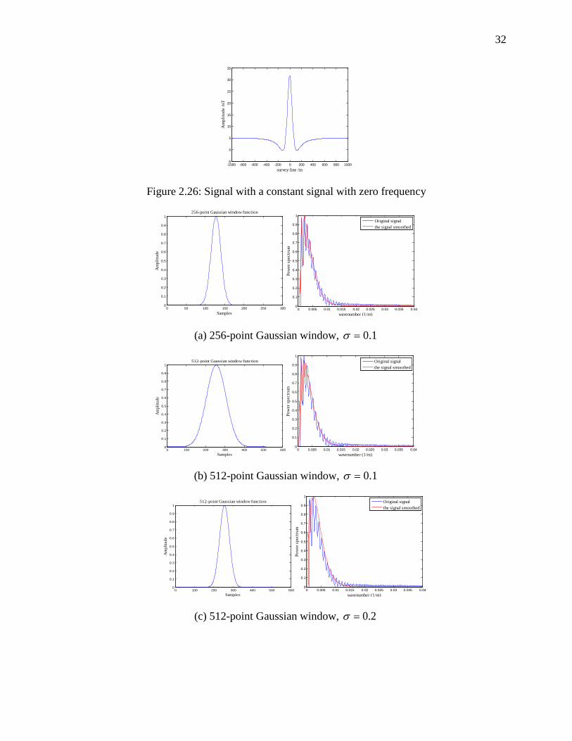
32
-1000 -800 -600 -400 -200 0 200 400 600 800 1000-5
0
5
10
15
20
25
30
35
Am
plitu
de /n
T
survey line /m
Figure 2.26: Signal with a constant signal with zero frequency
0 50 100 150 200 250 3000
0.1
0.2
0.3
0.4
0.5
0.6
0.7
0.8
0.9
1
Am
plitu
de
Samples
256-point Gaussian window function
0 0.005 0.01 0.015 0.02 0.025 0.03 0.035 0.040
0.1
0.2
0.3
0.4
0.5
0.6
0.7
0.8
0.9
1
Pow
er sp
ectru
m
wavenumber (1/m)
Original signalthe signal smoothed
(a) 256-point Gaussian window, 0.1σ =
0 100 200 300 400 500 6000
0.1
0.2
0.3
0.4
0.5
0.6
0.7
0.8
0.9
1
Ampl
itude
Samples
512-point Gaussian window function
0 0.005 0.01 0.015 0.02 0.025 0.03 0.035 0.040
0.1
0.2
0.3
0.4
0.5
0.6
0.7
0.8
0.9
1
Pow
er sp
ectru
m
wavenumber (1/m)
Original signalthe signal smoothed
(b) 512-point Gaussian window, 0.1σ =
0 100 200 300 400 500 6000
0.1
0.2
0.3
0.4
0.5
0.6
0.7
0.8
0.9
1
Ampl
itude
Samples
512-point Gaussian window function
0 0.005 0.01 0.015 0.02 0.025 0.03 0.035 0.040
0.1
0.2
0.3
0.4
0.5
0.6
0.7
0.8
0.9
1
Pow
er sp
ectru
m
wavenumber (1/m)
Original signalthe signal smoothed
(c) 512-point Gaussian window, 0.2σ =
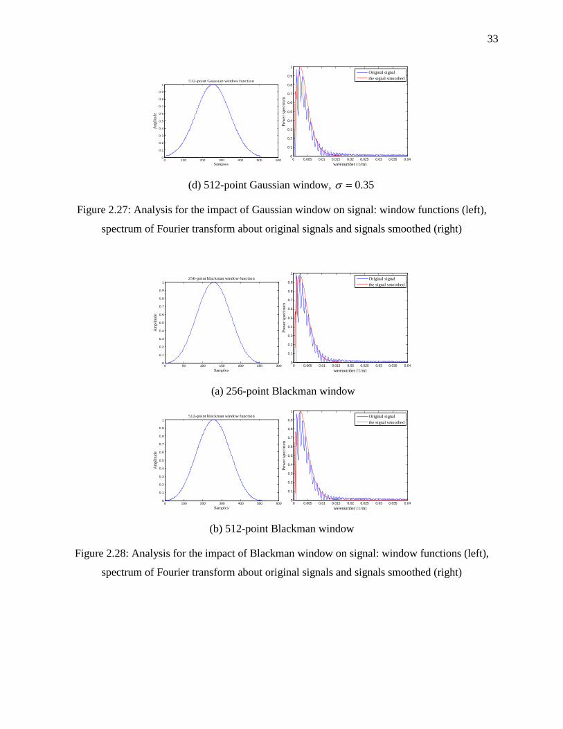
33
0 100 200 300 400 500 6000
0.1
0.2
0.3
0.4
0.5
0.6
0.7
0.8
0.9
1
Ampl
itude
Samples
512-point Gaussian window function
0 0.005 0.01 0.015 0.02 0.025 0.03 0.035 0.040
0.1
0.2
0.3
0.4
0.5
0.6
0.7
0.8
0.9
1
Pow
er sp
ectru
m
wavenumber (1/m)
Original signalthe signal smoothed
(d) 512-point Gaussian window, 0.35σ =
Figure 2.27: Analysis for the impact of Gaussian window on signal: window functions (left),
spectrum of Fourier transform about original signals and signals smoothed (right)
0 50 100 150 200 250 3000
0.1
0.2
0.3
0.4
0.5
0.6
0.7
0.8
0.9
1
Ampl
itude
Samples
256-point blackman window function
0 0.005 0.01 0.015 0.02 0.025 0.03 0.035 0.040
0.1
0.2
0.3
0.4
0.5
0.6
0.7
0.8
0.9
1
Pow
er sp
ectru
m
wavenumber (1/m)
Original signalthe signal smoothed
(a) 256-point Blackman window
0 100 200 300 400 500 6000
0.1
0.2
0.3
0.4
0.5
0.6
0.7
0.8
0.9
1
Ampl
itude
Samples
512-point blackman window function
0 0.005 0.01 0.015 0.02 0.025 0.03 0.035 0.040
0.1
0.2
0.3
0.4
0.5
0.6
0.7
0.8
0.9
1
Pow
er sp
ectru
m
wavenumber (1/m)
Original signalthe signal smoothed
(b) 512-point Blackman window
Figure 2.28: Analysis for the impact of Blackman window on signal: window functions (left),
spectrum of Fourier transform about original signals and signals smoothed (right)
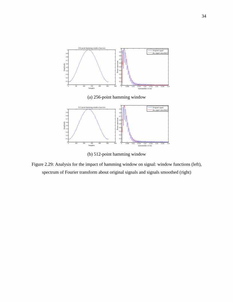
34
0 50 100 150 200 250 3000
0.1
0.2
0.3
0.4
0.5
0.6
0.7
0.8
0.9
1
Am
plitu
de
Samples
256-point hamming window function
0 0.005 0.01 0.015 0.02 0.025 0.03 0.035 0.040
0.1
0.2
0.3
0.4
0.5
0.6
0.7
0.8
0.9
1
Pow
er sp
ectru
m
wavenumber (1/m)
Original signalthe signal smoothed
(a) 256-point hamming window
0 100 200 300 400 500 6000
0.1
0.2
0.3
0.4
0.5
0.6
0.7
0.8
0.9
1
Am
plitu
de
Samples
512-point hamming window function
0 0.005 0.01 0.015 0.02 0.025 0.03 0.035 0.040
0.1
0.2
0.3
0.4
0.5
0.6
0.7
0.8
0.9
1
Pow
er sp
ectru
m
wavenumber (1/m)
Original signalthe signal smoothed
(b) 512-point hamming window
Figure 2.29: Analysis for the impact of hamming window on signal: window functions (left),
spectrum of Fourier transform about original signals and signals smoothed (right)
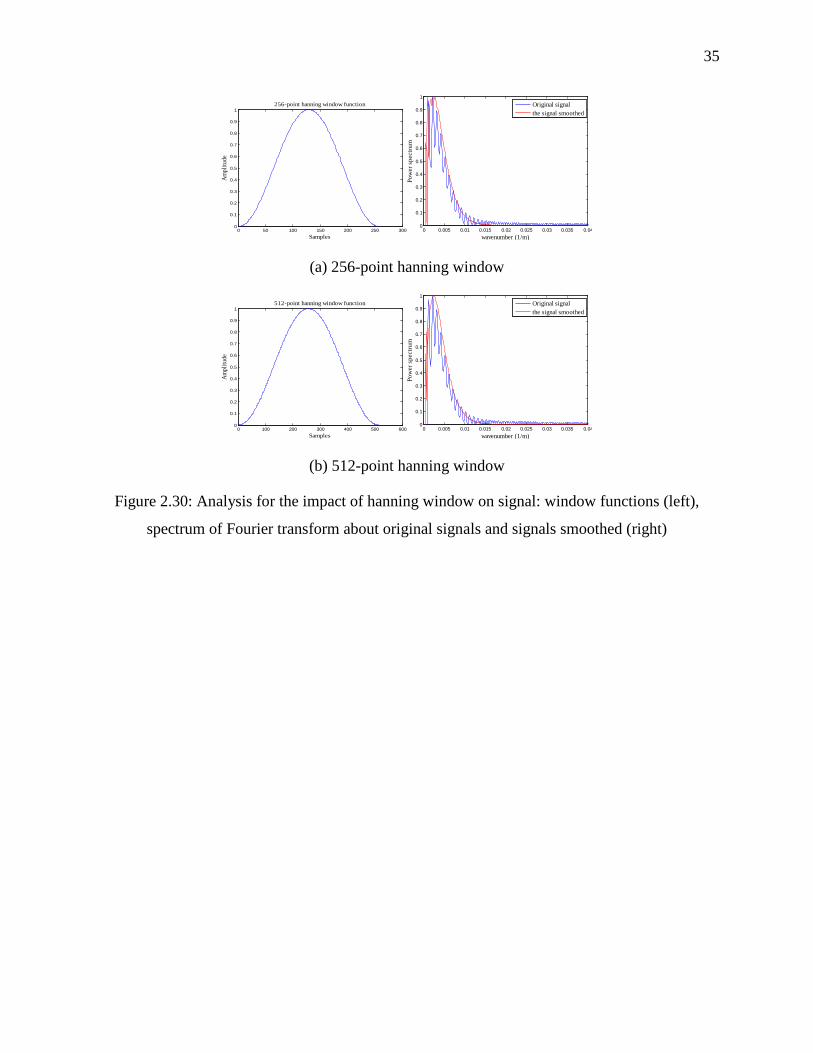
35
0 50 100 150 200 250 3000
0.1
0.2
0.3
0.4
0.5
0.6
0.7
0.8
0.9
1
Ampl
itude
Samples
256-point hanning window function
0 0.005 0.01 0.015 0.02 0.025 0.03 0.035 0.040
0.1
0.2
0.3
0.4
0.5
0.6
0.7
0.8
0.9
1
Pow
er sp
ectru
m
wavenumber (1/m)
Original signalthe signal smoothed
(a) 256-point hanning window
0 100 200 300 400 500 6000
0.1
0.2
0.3
0.4
0.5
0.6
0.7
0.8
0.9
1
Ampl
itude
Samples
512-point hanning window function
0 0.005 0.01 0.015 0.02 0.025 0.03 0.035 0.040
0.1
0.2
0.3
0.4
0.5
0.6
0.7
0.8
0.9
1
Pow
er sp
ectru
m
wavenumber (1/m)
Original signalthe signal smoothed
(b) 512-point hanning window
Figure 2.30: Analysis for the impact of hanning window on signal: window functions (left),
spectrum of Fourier transform about original signals and signals smoothed (right)
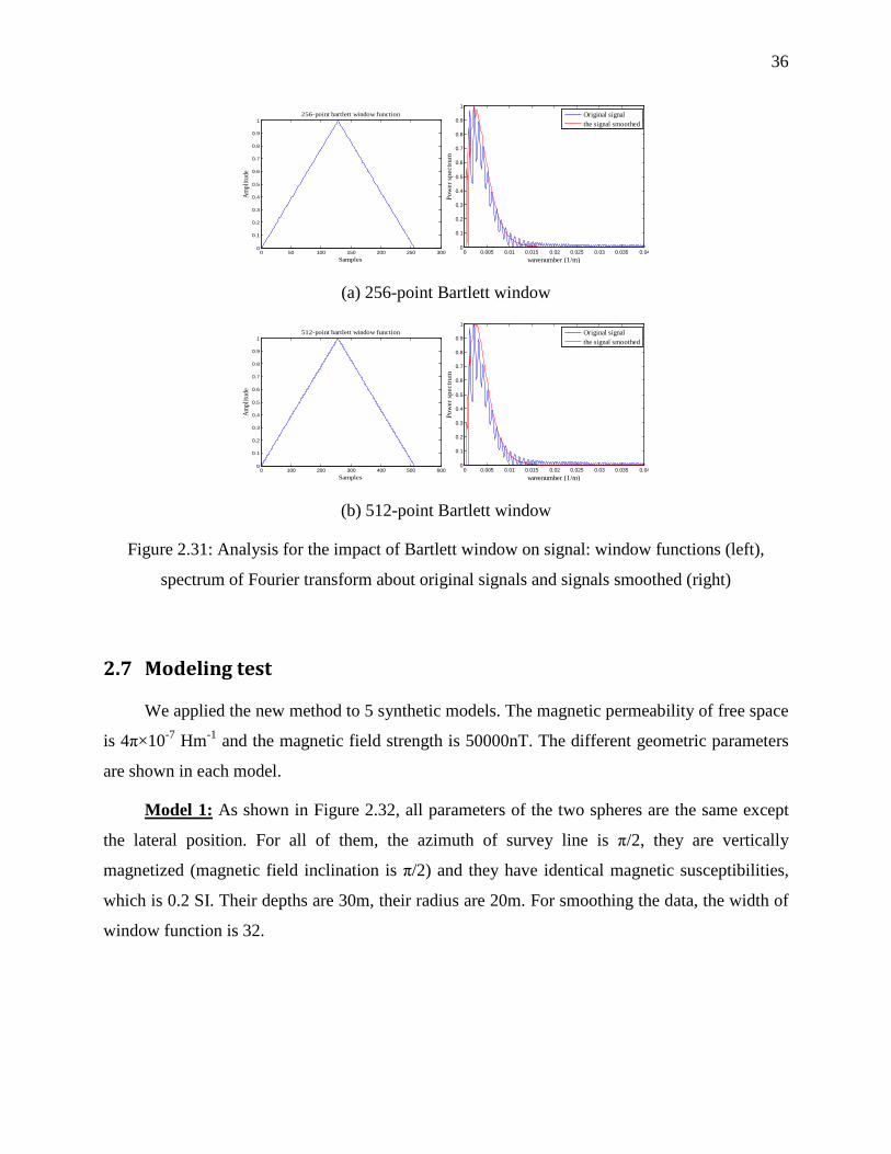
36
0 50 100 150 200 250 3000
0.1
0.2
0.3
0.4
0.5
0.6
0.7
0.8
0.9
1
Ampl
itude
Samples
256-point bartlett window function
0 0.005 0.01 0.015 0.02 0.025 0.03 0.035 0.040
0.1
0.2
0.3
0.4
0.5
0.6
0.7
0.8
0.9
1
Pow
er sp
ectru
m
wavenumber (1/m)
Original signalthe signal smoothed
(a) 256-point Bartlett window
0 100 200 300 400 500 6000
0.1
0.2
0.3
0.4
0.5
0.6
0.7
0.8
0.9
1
Ampl
itude
Samples
512-point bartlett window function
0 0.005 0.01 0.015 0.02 0.025 0.03 0.035 0.040
0.1
0.2
0.3
0.4
0.5
0.6
0.7
0.8
0.9
1
Pow
er sp
ectru
m
wavenumber (1/m)
Original signalthe signal smoothed
(b) 512-point Bartlett window
Figure 2.31: Analysis for the impact of Bartlett window on signal: window functions (left),
spectrum of Fourier transform about original signals and signals smoothed (right)
2.7 Modeling test
We applied the new method to 5 synthetic models. The magnetic permeability of free space
is 4π×10-7 Hm-1 and the magnetic field strength is 50000nT. The different geometric parameters
are shown in each model.
Model 1: As shown in Figure 2.32, all parameters of the two spheres are the same except
the lateral position. For all of them, the azimuth of survey line is π/2, they are vertically
magnetized (magnetic field inclination is π/2) and they have identical magnetic susceptibilities,
which is 0.2 SI. Their depths are 30m, their radius are 20m. For smoothing the data, the width of
window function is 32.
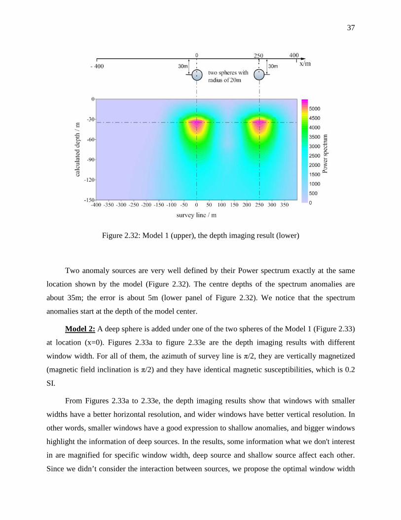
37
Figure 2.32: Model 1 (upper), the depth imaging result (lower)
Two anomaly sources are very well defined by their Power spectrum exactly at the same
location shown by the model (Figure 2.32). The centre depths of the spectrum anomalies are
about 35m; the error is about 5m (lower panel of Figure 2.32). We notice that the spectrum
anomalies start at the depth of the model center.
Model 2: A deep sphere is added under one of the two spheres of the Model 1 (Figure 2.33)
at location (x=0). Figures 2.33a to figure 2.33e are the depth imaging results with different
window width. For all of them, the azimuth of survey line is π/2, they are vertically magnetized
(magnetic field inclination is π/2) and they have identical magnetic susceptibilities, which is 0.2
SI.
From Figures 2.33a to 2.33e, the depth imaging results show that windows with smaller
widths have a better horizontal resolution, and wider windows have better vertical resolution. In
other words, smaller windows have a good expression to shallow anomalies, and bigger windows
highlight the information of deep sources. In the results, some information what we don't interest
in are magnified for specific window width, deep source and shallow source affect each other.
Since we didn’t consider the interaction between sources, we propose the optimal window width
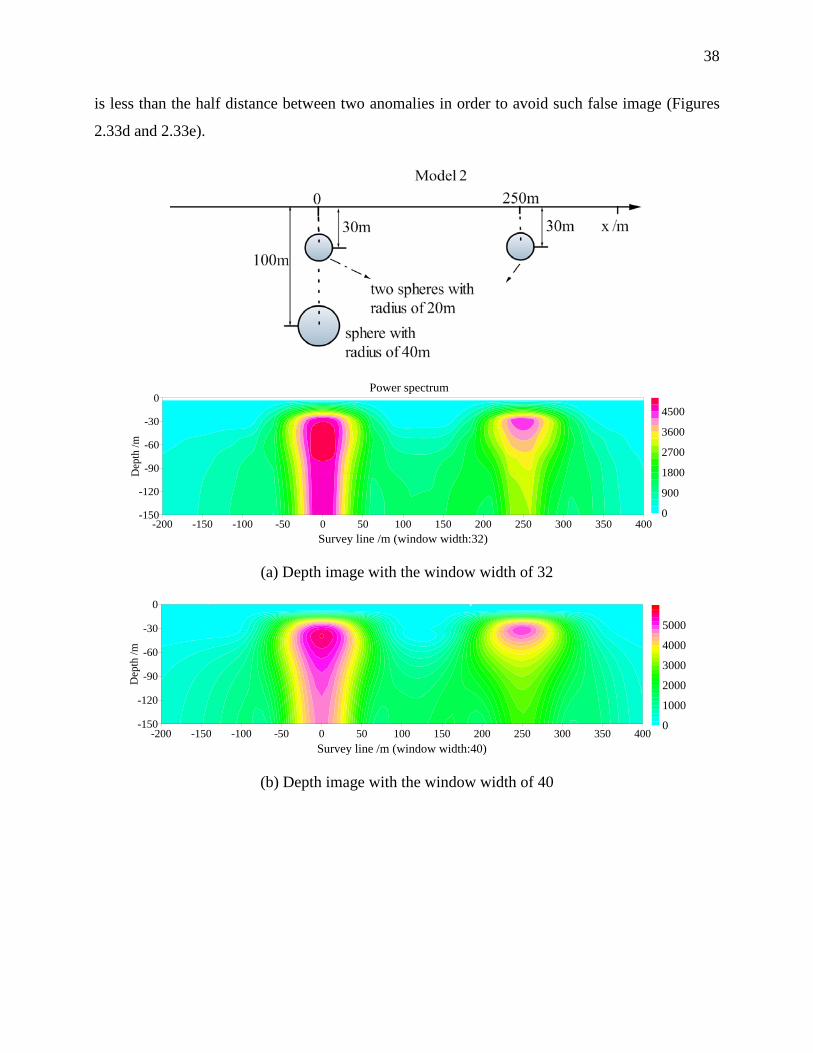
38
is less than the half distance between two anomalies in order to avoid such false image (Figures
2.33d and 2.33e).
-200 -150 -100 -50 0 50 100 150 200 250 300 350 400Survey line /m (window width:32)
-150
-120
-90
-60
-30
0
Dep
th /m
0
900
1800
2700
3600
4500
Power spectrum
(a) Depth image with the window width of 32
-200 -150 -100 -50 0 50 100 150 200 250 300 350 400Survey line /m (window width:40)
-150
-120
-90
-60
-30
0
Dep
th /m
0
1000
2000
3000
4000
5000
(b) Depth image with the window width of 40
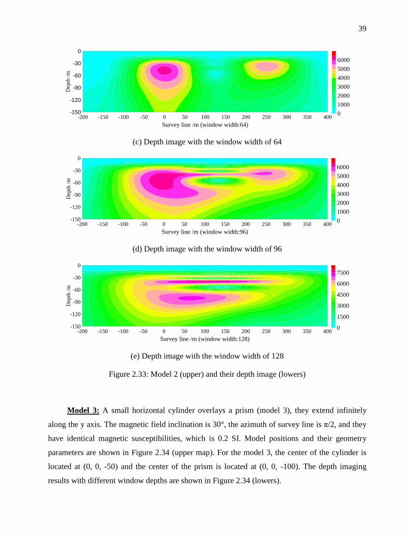
39
-200 -150 -100 -50 0 50 100 150 200 250 300 350 400Survey line /m (window width:64)
-150
-120
-90
-60
-30
0
Dep
th /m
0100020003000400050006000
(c) Depth image with the window width of 64
-200 -150 -100 -50 0 50 100 150 200 250 300 350 400Survey line /m (window width:96)
-150
-120
-90
-60
-30
0
Dep
th /m
0100020003000400050006000
(d) Depth image with the window width of 96
-200 -150 -100 -50 0 50 100 150 200 250 300 350 400Survey line /m (window width:128)
-150
-120
-90
-60
-30
0
Dep
th /m
0
1500
3000
4500
6000
7500
(e) Depth image with the window width of 128
Figure 2.33: Model 2 (upper) and their depth image (lowers)
Model 3: A small horizontal cylinder overlays a prism (model 3), they extend infinitely
along the y axis. The magnetic field inclination is 30°, the azimuth of survey line is π/2, and they
have identical magnetic susceptibilities, which is 0.2 SI. Model positions and their geometry
parameters are shown in Figure 2.34 (upper map). For the model 3, the center of the cylinder is
located at (0, 0, -50) and the center of the prism is located at (0, 0, -100). The depth imaging
results with different window depths are shown in Figure 2.34 (lowers).
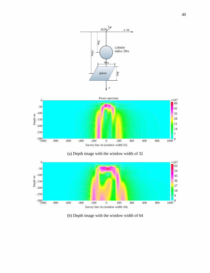
40
-1000 -800 -600 -400 -200 0 200 400 600 800 1000Survey line /m (window width:32)
-300
-250
-200
-150
-100
-50
0
Dep
th /m
07142128354249
Power spectrum ×103
(a) Depth image with the window width of 32
-1000 -800 -600 -400 -200 0 200 400 600 800 1000Survey line /m (window width: 64)
-300
-250
-200
-150
-100
-50
0
Dep
th /m
09182736455463
×103
(b) Depth image with the window width of 64
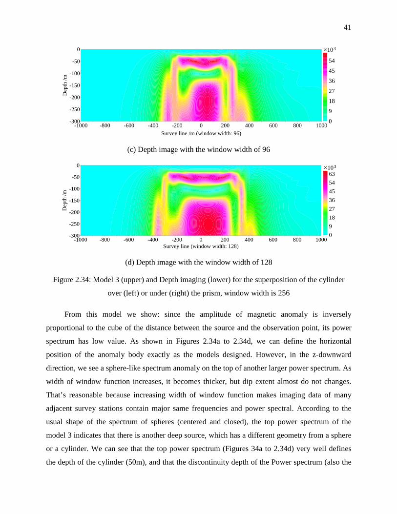
41
-1000 -800 -600 -400 -200 0 200 400 600 800 1000Survey line /m (window width: 96)
-300
-250
-200
-150
-100
-50
0
Dep
th /m
091827364554
×103
(c) Depth image with the window width of 96
-1000 -800 -600 -400 -200 0 200 400 600 800 1000Survey line (window width: 128)
-300
-250
-200
-150
-100
-50
0
Dep
th /m
09182736455463
×103
(d) Depth image with the window width of 128
Figure 2.34: Model 3 (upper) and Depth imaging (lower) for the superposition of the cylinder
over (left) or under (right) the prism, window width is 256
From this model we show: since the amplitude of magnetic anomaly is inversely
proportional to the cube of the distance between the source and the observation point, its power
spectrum has low value. As shown in Figures 2.34a to 2.34d, we can define the horizontal
position of the anomaly body exactly as the models designed. However, in the z-downward
direction, we see a sphere-like spectrum anomaly on the top of another larger power spectrum. As
width of window function increases, it becomes thicker, but dip extent almost do not changes.
That’s reasonable because increasing width of window function makes imaging data of many
adjacent survey stations contain major same frequencies and power spectral. According to the
usual shape of the spectrum of spheres (centered and closed), the top power spectrum of the
model 3 indicates that there is another deep source, which has a different geometry from a sphere
or a cylinder. We can see that the top power spectrum (Figures 34a to 2.34d) very well defines
the depth of the cylinder (50m), and that the discontinuity depth of the Power spectrum (also the
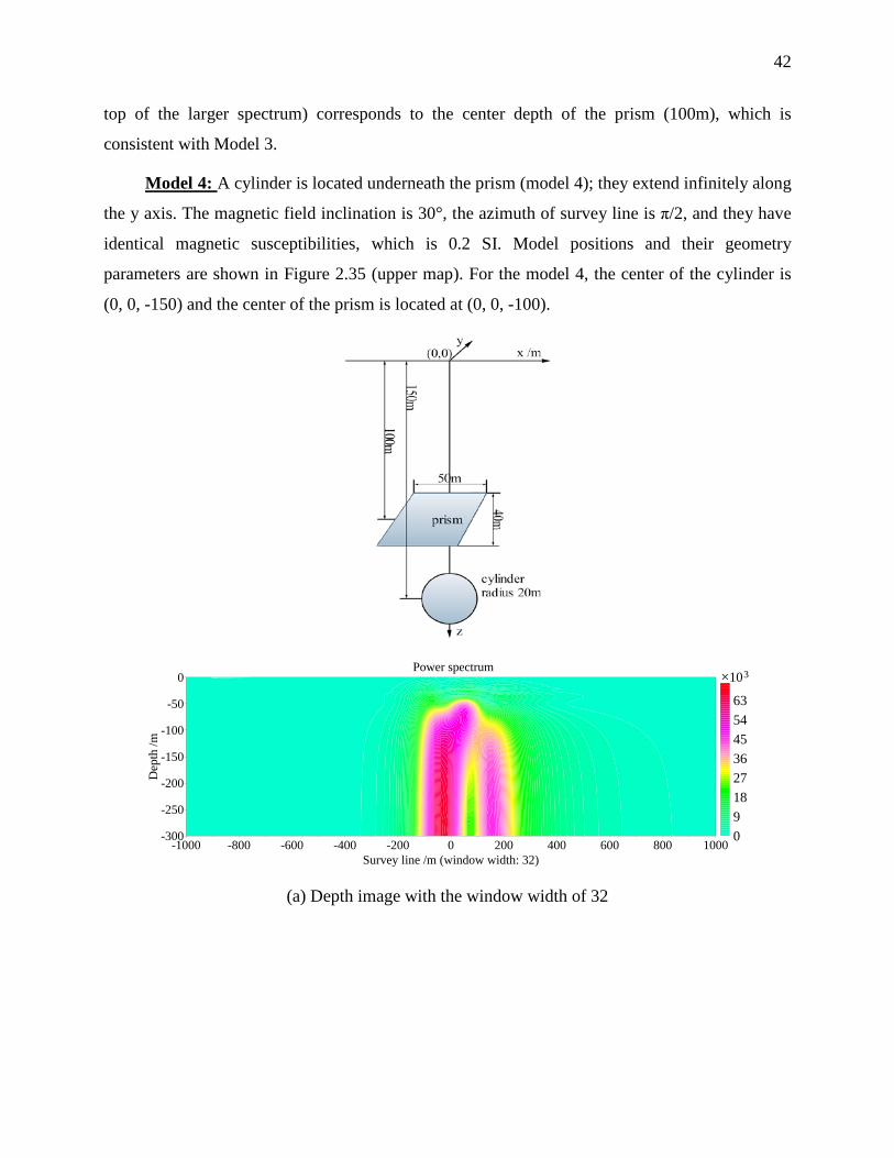
42
top of the larger spectrum) corresponds to the center depth of the prism (100m), which is
consistent with Model 3.
Model 4: A cylinder is located underneath the prism (model 4); they extend infinitely along
the y axis. The magnetic field inclination is 30°, the azimuth of survey line is π/2, and they have
identical magnetic susceptibilities, which is 0.2 SI. Model positions and their geometry
parameters are shown in Figure 2.35 (upper map). For the model 4, the center of the cylinder is
(0, 0, -150) and the center of the prism is located at (0, 0, -100).
-1000 -800 -600 -400 -200 0 200 400 600 800 1000Survey line /m (window width: 32)
-300
-250
-200
-150
-100
-50
0
Dep
th /m
Power spectrum
09182736455463
×103
(a) Depth image with the window width of 32
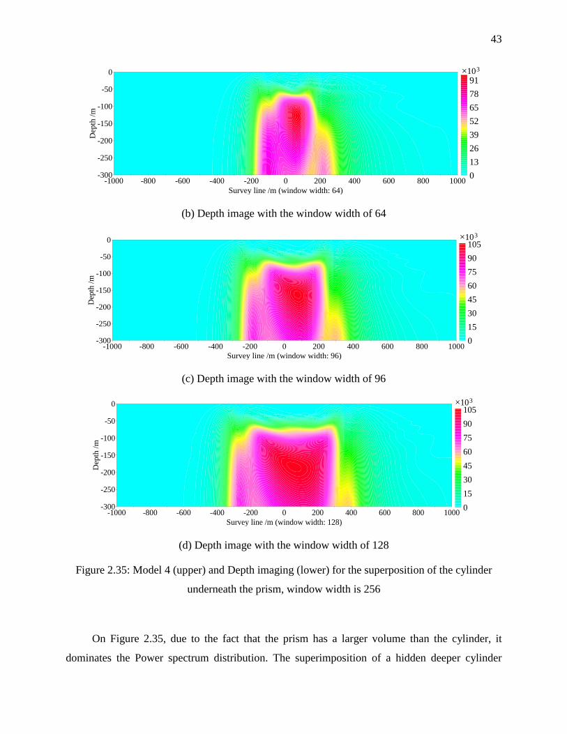
43
-1000 -800 -600 -400 -200 0 200 400 600 800 1000Survey line /m (window width: 64)
-300
-250
-200
-150
-100
-50
0
Dep
th /m
013263952657891
×103
(b) Depth image with the window width of 64
-1000 -800 -600 -400 -200 0 200 400 600 800 1000Survey line /m (window width: 96)
-300
-250
-200
-150
-100
-50
0
Dep
th /m
0153045607590105
×103
(c) Depth image with the window width of 96
-1000 -800 -600 -400 -200 0 200 400 600 800 1000Survey line /m (window width: 128)
-300
-250
-200
-150
-100
-50
0
Dep
th /m
0153045607590105
×103
(d) Depth image with the window width of 128
Figure 2.35: Model 4 (upper) and Depth imaging (lower) for the superposition of the cylinder
underneath the prism, window width is 256
On Figure 2.35, due to the fact that the prism has a larger volume than the cylinder, it
dominates the Power spectrum distribution. The superimposition of a hidden deeper cylinder
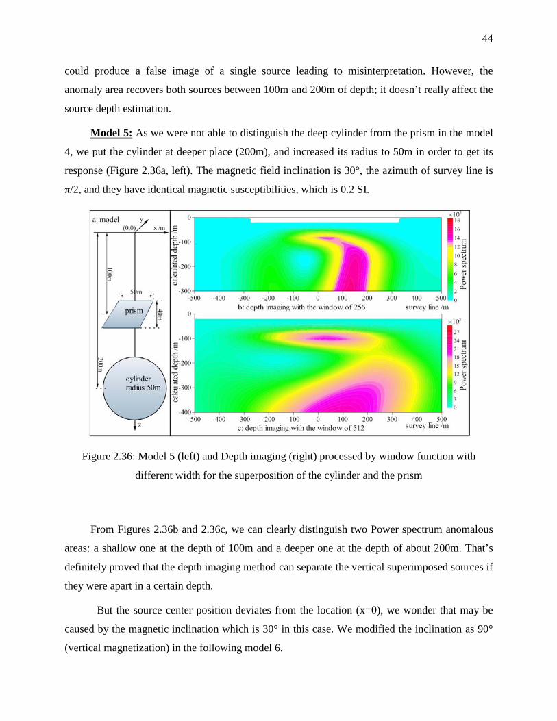
44
could produce a false image of a single source leading to misinterpretation. However, the
anomaly area recovers both sources between 100m and 200m of depth; it doesn’t really affect the
source depth estimation.
Model 5: As we were not able to distinguish the deep cylinder from the prism in the model
4, we put the cylinder at deeper place (200m), and increased its radius to 50m in order to get its
response (Figure 2.36a, left). The magnetic field inclination is 30°, the azimuth of survey line is
π/2, and they have identical magnetic susceptibilities, which is 0.2 SI.
Figure 2.36: Model 5 (left) and Depth imaging (right) processed by window function with
different width for the superposition of the cylinder and the prism
From Figures 2.36b and 2.36c, we can clearly distinguish two Power spectrum anomalous
areas: a shallow one at the depth of 100m and a deeper one at the depth of about 200m. That’s
definitely proved that the depth imaging method can separate the vertical superimposed sources if
they were apart in a certain depth.
But the source center position deviates from the location (x=0), we wonder that may be
caused by the magnetic inclination which is 30° in this case. We modified the inclination as 90°
(vertical magnetization) in the following model 6.
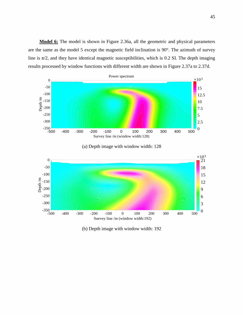
45
Model 6: The model is shown in Figure 2.36a, all the geometric and physical parameters
are the same as the model 5 except the magnetic field inclination is 90°. The azimuth of survey
line is π/2, and they have identical magnetic susceptibilities, which is 0.2 SI. The depth imaging
results processed by window functions with different width are shown in Figure 2.37a to 2.37d.
-500 -400 -300 -200 -100 0 100 200 300 400 500Survey line /m (window width:128)
Power spectrum
-350
-300
-250
-200
-150
-100
-50
0
Dep
th /m
02.557.51012.515
×103
(a) Depth image with window width: 128
-500 -400 -300 -200 -100 0 100 200 300 400 500Suevey line /m (window width:192)
-350
-300
-250
-200
-150
-100
-50
0
Dep
th /m
036912151821
×103
(b) Depth image with window width: 192
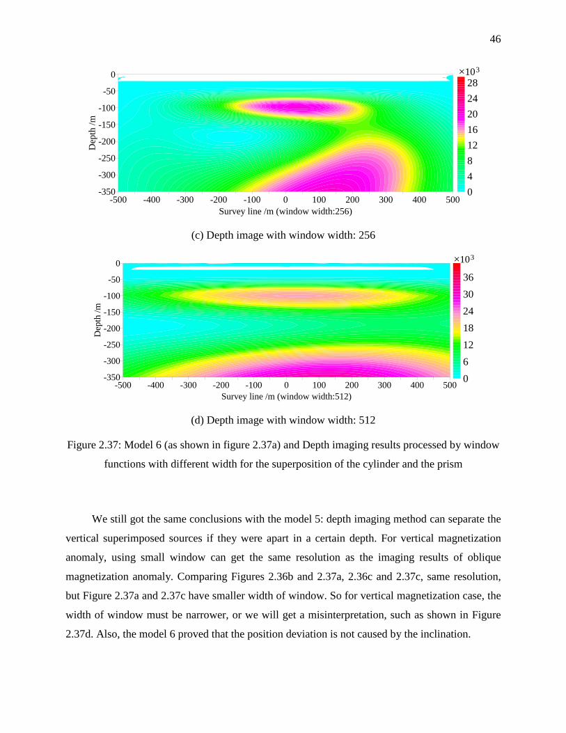
46
-500 -400 -300 -200 -100 0 100 200 300 400 500Survey line /m (window width:256)
-350
-300
-250
-200
-150
-100
-50
0
Dep
th /m
0481216202428
×103
(c) Depth image with window width: 256
-500 -400 -300 -200 -100 0 100 200 300 400 500Survey line /m (window width:512)
-350
-300
-250
-200
-150
-100
-50
0
Dep
th /m
061218243036
×103
(d) Depth image with window width: 512
Figure 2.37: Model 6 (as shown in figure 2.37a) and Depth imaging results processed by window
functions with different width for the superposition of the cylinder and the prism
We still got the same conclusions with the model 5: depth imaging method can separate the
vertical superimposed sources if they were apart in a certain depth. For vertical magnetization
anomaly, using small window can get the same resolution as the imaging results of oblique
magnetization anomaly. Comparing Figures 2.36b and 2.37a, 2.36c and 2.37c, same resolution,
but Figure 2.37a and 2.37c have smaller width of window. So for vertical magnetization case, the
width of window must be narrower, or we will get a misinterpretation, such as shown in Figure
2.37d. Also, the model 6 proved that the position deviation is not caused by the inclination.
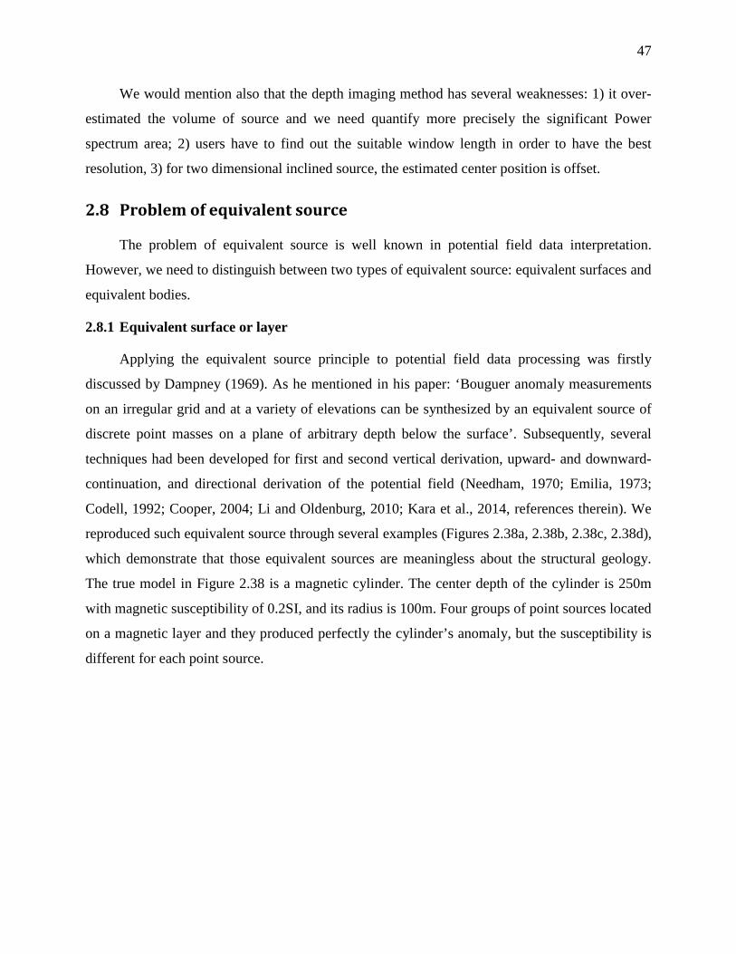
47
We would mention also that the depth imaging method has several weaknesses: 1) it over-
estimated the volume of source and we need quantify more precisely the significant Power
spectrum area; 2) users have to find out the suitable window length in order to have the best
resolution, 3) for two dimensional inclined source, the estimated center position is offset.
2.8 Problem of equivalent source
The problem of equivalent source is well known in potential field data interpretation.
However, we need to distinguish between two types of equivalent source: equivalent surfaces and
equivalent bodies.
2.8.1 Equivalent surface or layer
Applying the equivalent source principle to potential field data processing was firstly
discussed by Dampney (1969). As he mentioned in his paper: ‘Bouguer anomaly measurements
on an irregular grid and at a variety of elevations can be synthesized by an equivalent source of
discrete point masses on a plane of arbitrary depth below the surface’. Subsequently, several
techniques had been developed for first and second vertical derivation, upward- and downward-
continuation, and directional derivation of the potential field (Needham, 1970; Emilia, 1973;
Codell, 1992; Cooper, 2004; Li and Oldenburg, 2010; Kara et al., 2014, references therein). We
reproduced such equivalent source through several examples (Figures 2.38a, 2.38b, 2.38c, 2.38d),
which demonstrate that those equivalent sources are meaningless about the structural geology.
The true model in Figure 2.38 is a magnetic cylinder. The center depth of the cylinder is 250m
with magnetic susceptibility of 0.2SI, and its radius is 100m. Four groups of point sources located
on a magnetic layer and they produced perfectly the cylinder’s anomaly, but the susceptibility is
different for each point source.
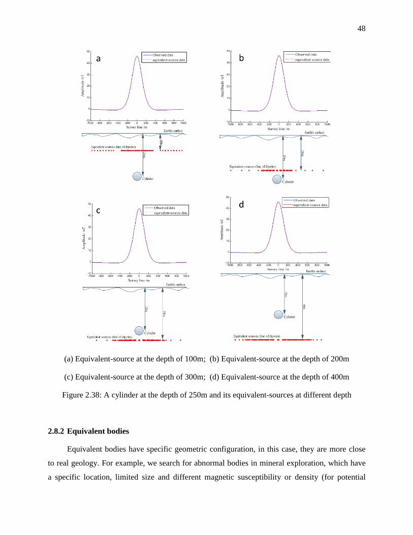
48
(a) Equivalent-source at the depth of 100m; (b) Equivalent-source at the depth of 200m
(c) Equivalent-source at the depth of 300m; (d) Equivalent-source at the depth of 400m
Figure 2.38: A cylinder at the depth of 250m and its equivalent-sources at different depth
2.8.2 Equivalent bodies
Equivalent bodies have specific geometric configuration, in this case, they are more close
to real geology. For example, we search for abnormal bodies in mineral exploration, which have
a specific location, limited size and different magnetic susceptibility or density (for potential
49
field) compared to surrounding rocks. The anomaly that is used in the interpretation represents
mostly the local geological feature. If there were several abnormal bodies who might produce a
same observed anomaly individually, this kind of equivalent source problem is totally different
from the equivalent surface. The latter is to find an arbitrary mass distribution which generates a
fixed potential, but the former is the problem to find the equal ratio of the magnetization or
density and the distance between the observation point and the abnormal body. In order to study
this type of equivalent sources, we did a series of modeling works and chosen several best fit
models that are shown in the Table 2.4.
We design a shallow prism model (prism 1) and use its magnetic anomaly as our reference
(red line on Figure 2.39). The survey line is E-W oriented and the strike direction of prism 1 is in
the N-S direction. If there is an equivalent source which is deeper than the prism 1, in order to
produce the same anomaly it should have higher susceptibility. At the depth of 200m, prism 2
and 3 (brown and green line respectively) show that the susceptibility has to be 10 times higher
than that of the prism 1 to reach the same amplitude of the anomaly. Due to the effect of depth,
they have larger width of the anomaly. Even we reduced the thickness of the prism 3 and
compensated the amplitude of anomaly by extending its vertical length from 300m to 500m; its
magnetic anomaly is still broader than the prism 1. We conclude that there is no such equivalent
body from the point of view of petrophysics and geology, because the maximum of the magnetic
susceptibility of Magnetite is 5.6 SI; of the Iron is 3.9 SI; of the pyrrhotite are 1.4 SI; of
Maghemite is 2.5 SI and of Ilmentite is 3.8 SI (PP Handbook, Peter Blum, 1997). We inclined the
prism 4 and 5 to see if the dip direction of prism makes impact on the anomaly. Indeed, it mostly
affects the shape of the anomaly not the amplitude.
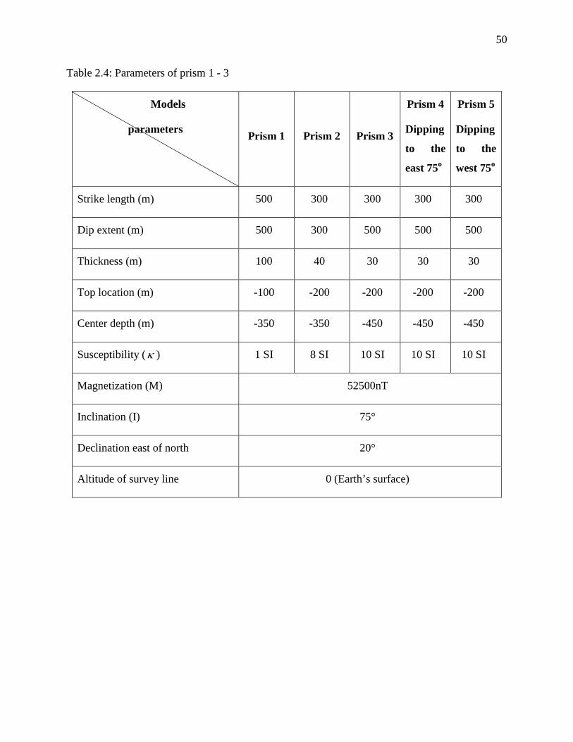
50
Table 2.4: Parameters of prism 1 - 3
Models
parameters Prism 1 Prism 2 Prism 3
Prism 4
Dipping
to the
east 75o
Prism 5
Dipping
to the
west 75o
Strike length (m) 500 300 300 300 300
Dip extent (m) 500 300 500 500 500
Thickness (m) 100 40 30 30 30
Top location (m) -100 -200 -200 -200 -200
Center depth (m) -350 -350 -450 -450 -450
Susceptibility (κ ) 1 SI 8 SI 10 SI 10 SI 10 SI
Magnetization (M) 52500nT
Inclination (I) 75°
Declination east of north 20°
Altitude of survey line 0 (Earth’s surface)
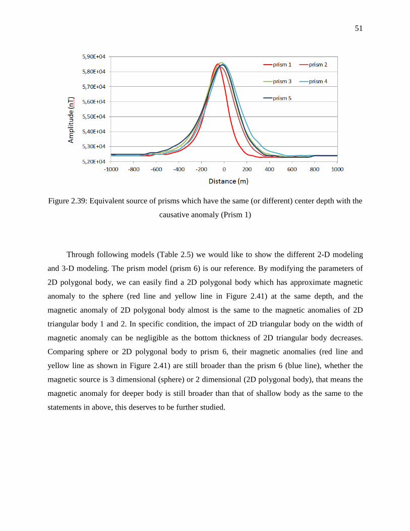
51
Figure 2.39: Equivalent source of prisms which have the same (or different) center depth with the
causative anomaly (Prism 1)
Through following models (Table 2.5) we would like to show the different 2-D modeling
and 3-D modeling. The prism model (prism 6) is our reference. By modifying the parameters of
2D polygonal body, we can easily find a 2D polygonal body which has approximate magnetic
anomaly to the sphere (red line and yellow line in Figure 2.41) at the same depth, and the
magnetic anomaly of 2D polygonal body almost is the same to the magnetic anomalies of 2D
triangular body 1 and 2. In specific condition, the impact of 2D triangular body on the width of
magnetic anomaly can be negligible as the bottom thickness of 2D triangular body decreases.
Comparing sphere or 2D polygonal body to prism 6, their magnetic anomalies (red line and
yellow line as shown in Figure 2.41) are still broader than the prism 6 (blue line), whether the
magnetic source is 3 dimensional (sphere) or 2 dimensional (2D polygonal body), that means the
magnetic anomaly for deeper body is still broader than that of shallow body as the same to the
statements in above, this deserves to be further studied.
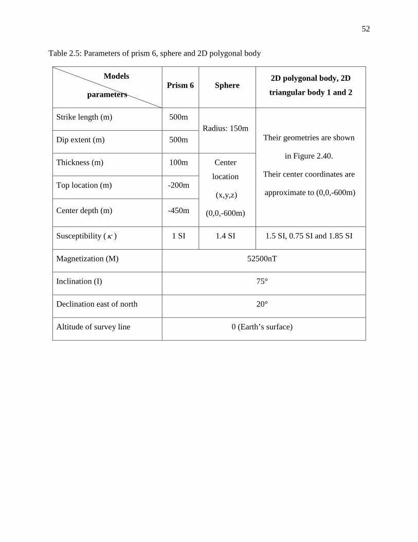
52
Table 2.5: Parameters of prism 6, sphere and 2D polygonal body
Models
parameters Prism 6 Sphere
2D polygonal body, 2D
triangular body 1 and 2
Strike length (m) 500m Radius: 150m
Their geometries are shown
in Figure 2.40.
Their center coordinates are
approximate to (0,0,-600m)
Dip extent (m) 500m
Thickness (m) 100m Center
location
(x,y,z)
(0,0,-600m)
Top location (m) -200m
Center depth (m) -450m
Susceptibility (κ ) 1 SI 1.4 SI 1.5 SI, 0.75 SI and 1.85 SI
Magnetization (M) 52500nT
Inclination (I) 75°
Declination east of north 20°
Altitude of survey line 0 (Earth’s surface)
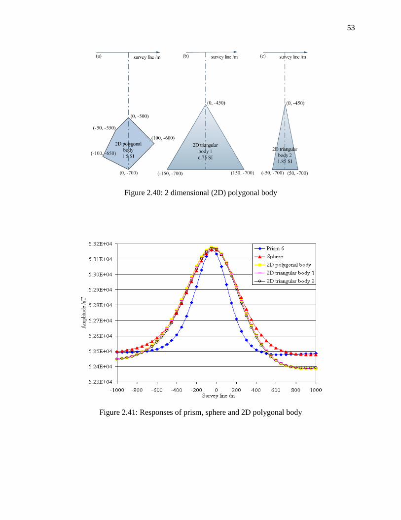
53
Figure 2.40: 2 dimensional (2D) polygonal body
Figure 2.41: Responses of prism, sphere and 2D polygonal body
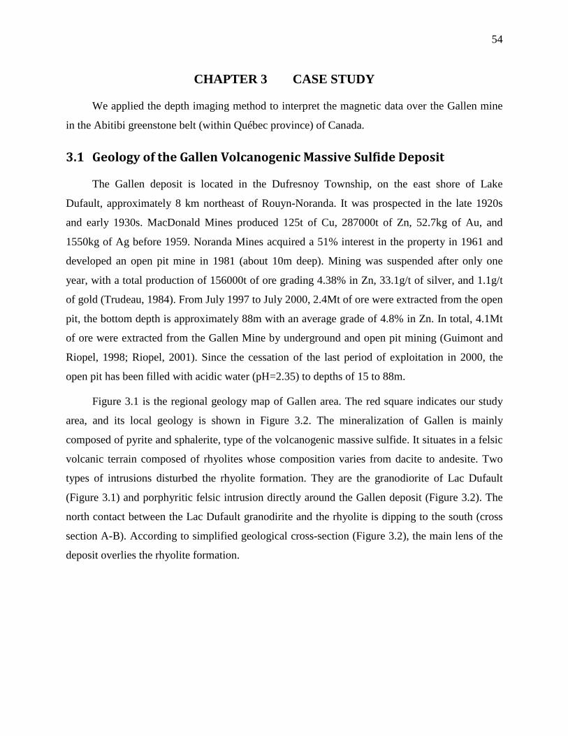
54
CHAPTER 3 CASE STUDY
We applied the depth imaging method to interpret the magnetic data over the Gallen mine
in the Abitibi greenstone belt (within Québec province) of Canada.
3.1 Geology of the Gallen Volcanogenic Massive Sulfide Deposit
The Gallen deposit is located in the Dufresnoy Township, on the east shore of Lake
Dufault, approximately 8 km northeast of Rouyn-Noranda. It was prospected in the late 1920s
and early 1930s. MacDonald Mines produced 125t of Cu, 287000t of Zn, 52.7kg of Au, and
1550kg of Ag before 1959. Noranda Mines acquired a 51% interest in the property in 1961 and
developed an open pit mine in 1981 (about 10m deep). Mining was suspended after only one
year, with a total production of 156000t of ore grading 4.38% in Zn, 33.1g/t of silver, and 1.1g/t
of gold (Trudeau, 1984). From July 1997 to July 2000, 2.4Mt of ore were extracted from the open
pit, the bottom depth is approximately 88m with an average grade of 4.8% in Zn. In total, 4.1Mt
of ore were extracted from the Gallen Mine by underground and open pit mining (Guimont and
Riopel, 1998; Riopel, 2001). Since the cessation of the last period of exploitation in 2000, the
open pit has been filled with acidic water (pH=2.35) to depths of 15 to 88m.
Figure 3.1 is the regional geology map of Gallen area. The red square indicates our study
area, and its local geology is shown in Figure 3.2. The mineralization of Gallen is mainly
composed of pyrite and sphalerite, type of the volcanogenic massive sulfide. It situates in a felsic
volcanic terrain composed of rhyolites whose composition varies from dacite to andesite. Two
types of intrusions disturbed the rhyolite formation. They are the granodiorite of Lac Dufault
(Figure 3.1) and porphyritic felsic intrusion directly around the Gallen deposit (Figure 3.2). The
north contact between the Lac Dufault granodirite and the rhyolite is dipping to the south (cross
section A-B). According to simplified geological cross-section (Figure 3.2), the main lens of the
deposit overlies the rhyolite formation.

55
Figure 3.1: Regional geology map of the Gallen area (Cheng et al., 2007).
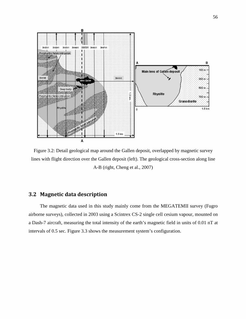
56
Figure 3.2: Detail geological map around the Gallen deposit, overlapped by magnetic survey
lines with flight direction over the Gallen deposit (left). The geological cross-section along line
A-B (right, Cheng et al., 2007)
3.2 Magnetic data description
The magnetic data used in this study mainly come from the MEGATEMII survey (Fugro
airborne surveys), collected in 2003 using a Scintrex CS-2 single cell cesium vapour, mounted on
a Dash-7 aircraft, measuring the total intensity of the earth’s magnetic field in units of 0.01 nT at
intervals of 0.5 sec. Figure 3.3 shows the measurement system’s configuration.
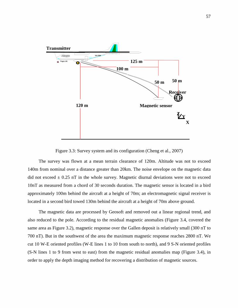
57
Figure 3.3: Survey system and its configuration (Cheng et al., 2007)
The survey was flown at a mean terrain clearance of 120m. Altitude was not to exceed
140m from nominal over a distance greater than 20km. The noise envelope on the magnetic data
did not exceed ± 0.25 nT in the whole survey. Magnetic diurnal deviations were not to exceed
10nT as measured from a chord of 30 seconds duration. The magnetic sensor is located in a bird
approximately 100m behind the aircraft at a height of 70m; an electromagnetic signal receiver is
located in a second bird towed 130m behind the aircraft at a height of 70m above ground.
The magnetic data are processed by Geosoft and removed out a linear regional trend, and
also reduced to the pole. According to the residual magnetic anomalies (Figure 3.4, covered the
same area as Figure 3.2), magnetic response over the Gallen deposit is relatively small (300 nT to
700 nT). But in the southwest of the area the maximum magnetic response reaches 2800 nT. We
cut 10 W-E oriented profiles (W-E lines 1 to 10 from south to north), and 9 S-N oriented profiles
(S-N lines 1 to 9 from west to east) from the magnetic residual anomalies map (Figure 3.4), in
order to apply the depth imaging method for recovering a distribution of magnetic sources.
125 m
Receiver
Transmitter
Fugro AS VH-TEM
50 m
120 m
Z
X Y
Magnetic sensor
50 m
100 m
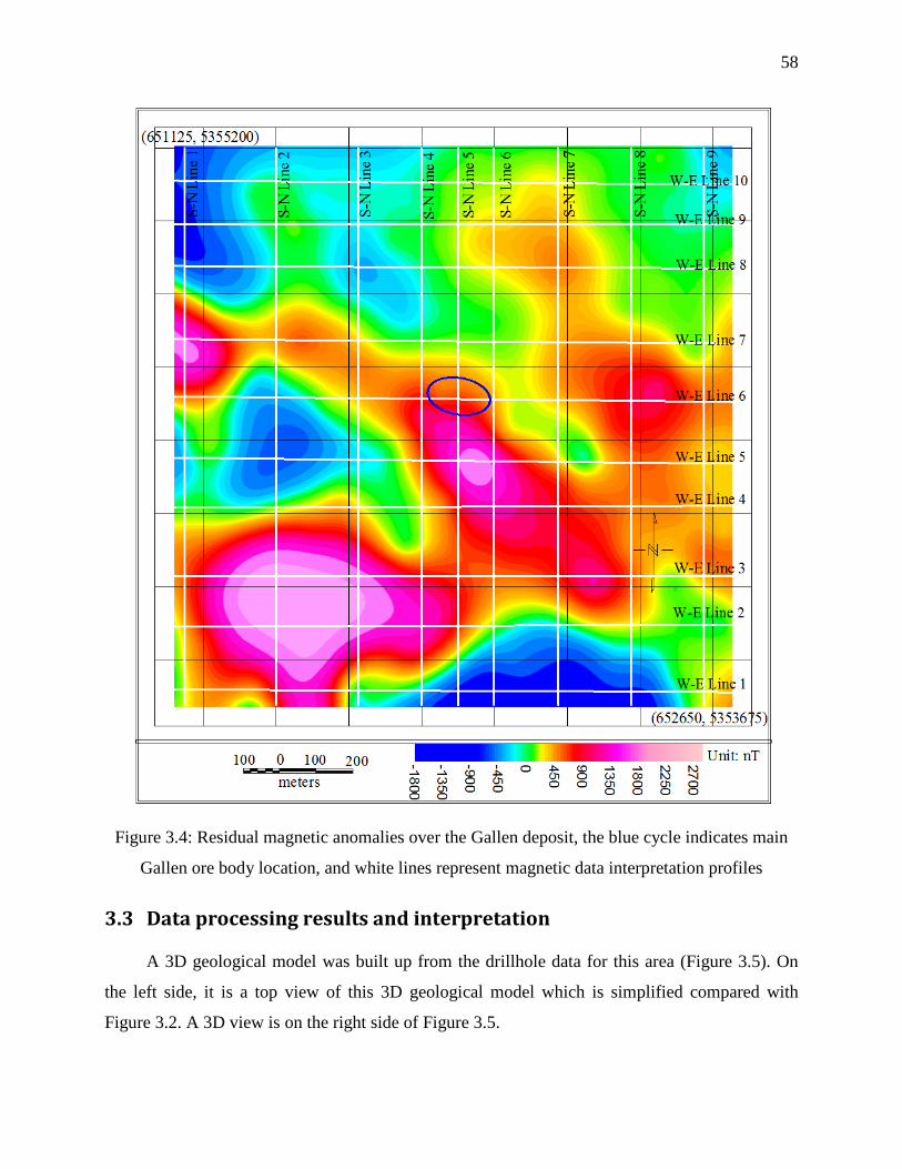
58
Figure 3.4: Residual magnetic anomalies over the Gallen deposit, the blue cycle indicates main
Gallen ore body location, and white lines represent magnetic data interpretation profiles
3.3 Data processing results and interpretation
A 3D geological model was built up from the drillhole data for this area (Figure 3.5). On
the left side, it is a top view of this 3D geological model which is simplified compared with
Figure 3.2. A 3D view is on the right side of Figure 3.5.
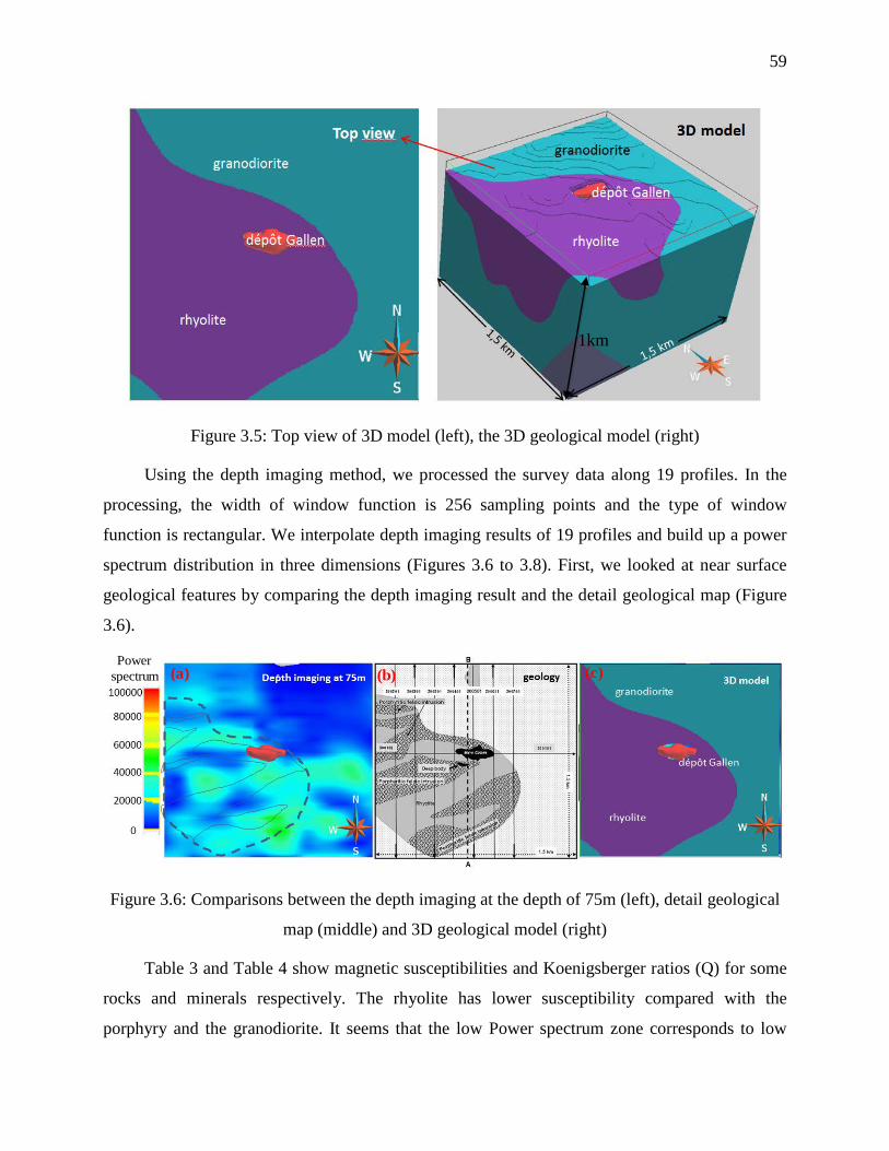
59
Figure 3.5: Top view of 3D model (left), the 3D geological model (right)
Using the depth imaging method, we processed the survey data along 19 profiles. In the
processing, the width of window function is 256 sampling points and the type of window
function is rectangular. We interpolate depth imaging results of 19 profiles and build up a power
spectrum distribution in three dimensions (Figures 3.6 to 3.8). First, we looked at near surface
geological features by comparing the depth imaging result and the detail geological map (Figure
3.6).
Power spectrum (a) (b) (c)
Figure 3.6: Comparisons between the depth imaging at the depth of 75m (left), detail geological
map (middle) and 3D geological model (right)
Table 3 and Table 4 show magnetic susceptibilities and Koenigsberger ratios (Q) for some
rocks and minerals respectively. The rhyolite has lower susceptibility compared with the
porphyry and the granodiorite. It seems that the low Power spectrum zone corresponds to low
1km
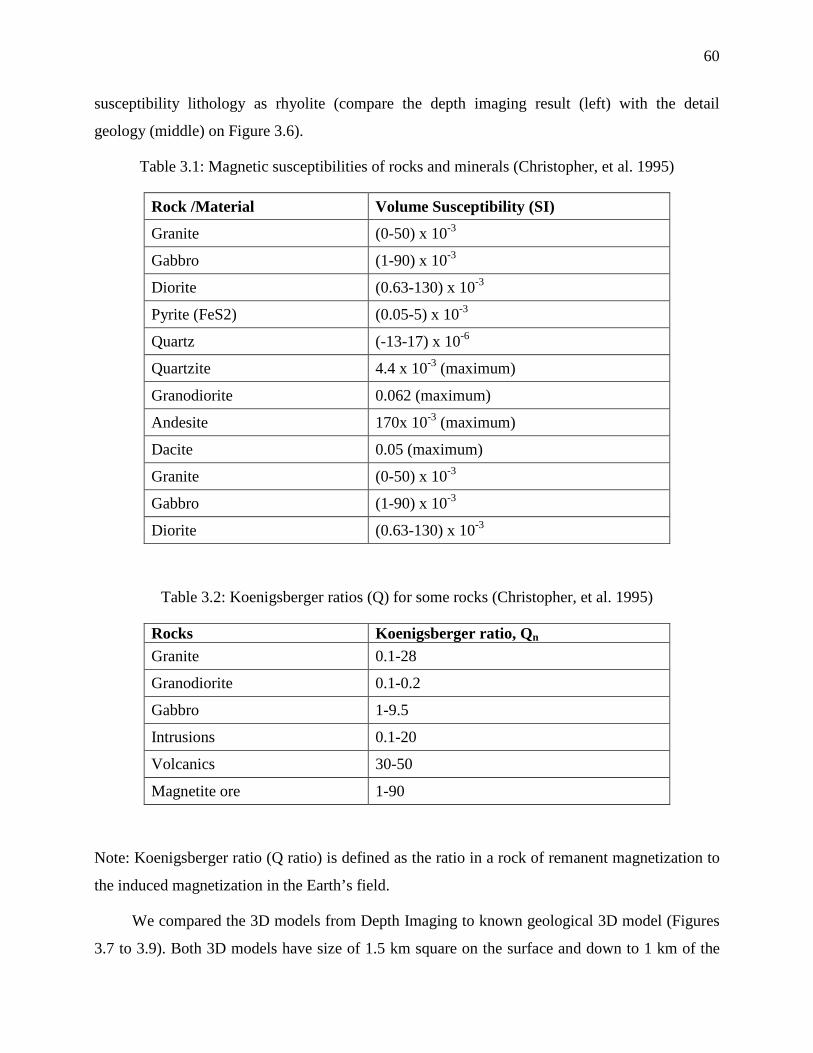
60
susceptibility lithology as rhyolite (compare the depth imaging result (left) with the detail
geology (middle) on Figure 3.6).
Table 3.1: Magnetic susceptibilities of rocks and minerals (Christopher, et al. 1995)
Rock /Material Volume Susceptibility (SI)
Granite (0-50) x 10-3
Gabbro (1-90) x 10-3
Diorite (0.63-130) x 10-3
Pyrite (FeS2) (0.05-5) x 10-3
Quartz (-13-17) x 10-6
Quartzite 4.4 x 10⁻³ (maximum)
Granodiorite 0.062 (maximum)
Andesite 170x 10-3 (maximum)
Dacite 0.05 (maximum)
Granite (0-50) x 10-3
Gabbro (1-90) x 10-3
Diorite (0.63-130) x 10-3
Table 3.2: Koenigsberger ratios (Q) for some rocks (Christopher, et al. 1995)
Rocks Koenigsberger ratio, Qn Granite 0.1-28
Granodiorite 0.1-0.2
Gabbro 1-9.5
Intrusions 0.1-20
Volcanics 30-50
Magnetite ore 1-90
Note: Koenigsberger ratio (Q ratio) is defined as the ratio in a rock of remanent magnetization to
the induced magnetization in the Earth’s field.
We compared the 3D models from Depth Imaging to known geological 3D model (Figures
3.7 to 3.9). Both 3D models have size of 1.5 km square on the surface and down to 1 km of the
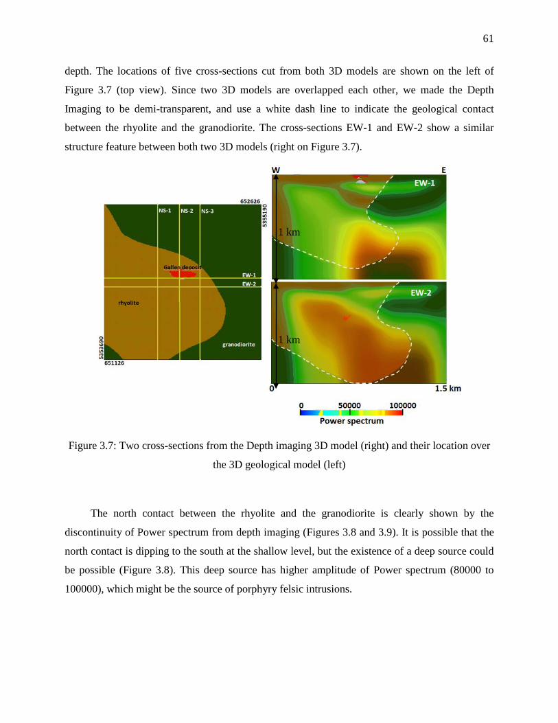
61
depth. The locations of five cross-sections cut from both 3D models are shown on the left of
Figure 3.7 (top view). Since two 3D models are overlapped each other, we made the Depth
Imaging to be demi-transparent, and use a white dash line to indicate the geological contact
between the rhyolite and the granodiorite. The cross-sections EW-1 and EW-2 show a similar
structure feature between both two 3D models (right on Figure 3.7).
Figure 3.7: Two cross-sections from the Depth imaging 3D model (right) and their location over
the 3D geological model (left)
The north contact between the rhyolite and the granodiorite is clearly shown by the
discontinuity of Power spectrum from depth imaging (Figures 3.8 and 3.9). It is possible that the
north contact is dipping to the south at the shallow level, but the existence of a deep source could
be possible (Figure 3.8). This deep source has higher amplitude of Power spectrum (80000 to
100000), which might be the source of porphyry felsic intrusions.
1 km
1 km
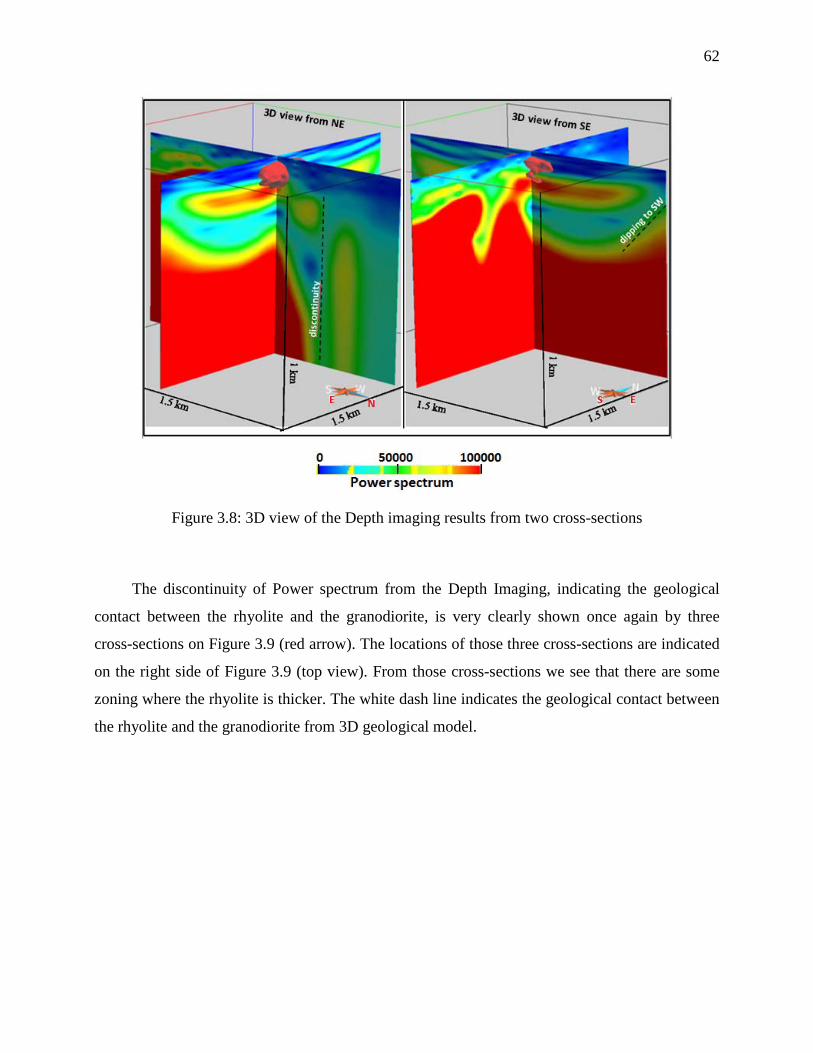
62
Figure 3.8: 3D view of the Depth imaging results from two cross-sections
The discontinuity of Power spectrum from the Depth Imaging, indicating the geological
contact between the rhyolite and the granodiorite, is very clearly shown once again by three
cross-sections on Figure 3.9 (red arrow). The locations of those three cross-sections are indicated
on the right side of Figure 3.9 (top view). From those cross-sections we see that there are some
zoning where the rhyolite is thicker. The white dash line indicates the geological contact between
the rhyolite and the granodiorite from 3D geological model.
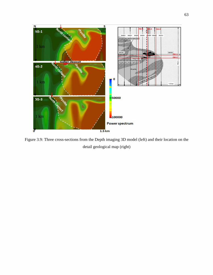
63
Figure 3.9: Three cross-sections from the Depth imaging 3D model (left) and their location on the
detail geological map (right)
1 km
1 km
1 km
64
CONCLUSION
We studied the characteristics of the Power spectrum of magnetic field anomalies in the
frequency domain and found that the spectrum of the anomaly is correlated with the depth of the
source of the anomaly. We deduced a mathematical formula to express the relation between the
depth and the wave number for a simple magnetic body. We extended this formula to a general
situation and got a depth imaging method to interpret magnetic data in term of distribution of
sources.
Using synthetic models, we tested this new method. For horizontal sources which are
separated away in horizontal direction, we can estimate the depth of a body with a high spatial
resolution. As the depth increases, higher accuracy is obtained regarding the depth estimation
from the Power spectrum. For vertical superposed bodies, we can image the depth at the top of
the deeper body. If a small body overlays a larger body, they can easily be separated by the
discontinuity of their spectrum in the depth; however, when the bigger body overlays a small one,
the top depth of the deepest body can be clearly determined only if they are separated by a certain
distance.
For magnetic anomaly, the noise may cause a gross distortion to the result of Fourier
transform as the NSR (the noise-signal ratio) increases, also the DC components become more
significant. The impact of noise on the component with small wavenumber is smaller than that
with bigger wavenumber for the peer noise-signal ratio.
For the problem of equivalent source, according to our studies it is possible that several
magnetic bodies at the same depth can produce same magnetic anomalies. However, it only
affects the form of the causative body without affecting the precise positioning of the source
which is the most important factor in mineral exploration. For a vertical stack of several magnetic
bodies, the depth impact on the shape of the magnetic anomaly cannot be compensated by the
variation of reasonable susceptibility values. In addition, when the depth of abnormal body
changes, the shape of magnetic anomaly also changes accordingly; therefore it is possible to
distinguish the body to different depths by our new method.
The effect of the edge in the Fourier transform (the Gibbs phenomenon) was considered in
our calculation. By using windows to smooth the signal, the results of Fourier transform are
65
much better than that of original signal. The principle to choose the window is that enough
number of sampling points and adjusting the parameters of window function make the original
signal smoother to zeros. Also the sampling points of window function do not be countless so
that it affects the computing speed.
Through the case study of Gallen, we showed also that the depth imaging method can
produce a complex model without any constraint of discretization of the model. We will continue
to work in the future towards more complex geological situations by adding known information
to improve spatial resolution. We also continue to find out the intrinsic link between the Power
spectrum and physical properties such as the magnetic susceptibility.
66
REFERENCES
ALLDREDGE LR. (1981). Rectangular harmonic analysis applied to the geomagnetic field. JGR,
86, 3021-3026.
AMALENDU Roy. 1962. Ambiguity in geophysical interpretation. Geophysics, XXXVII (1), 90-
99.
BACKUS G., GILBERT F. (1970). Uniqueness in the inversion of inaccurate gross earth data.
Phil. Trans. R. Soc., A266 (1173), 123-192.
BARNETT, C. T. (1976). Theoretical modeling of the magnetic and gravitational fields of an
arbitrarily shaped three-dimensional body. Geophysics, 41, 1353-1364.
BARTON, D. C.. (1929). Calculations in the interpretation of observations with the Eotvos
torsion balance. AIME, 481-486.
BERG E. (1990). Simple convergent genetic algorithm for inversion of multi parameter data.
60th SEG Annual Meeting. 948-945.
BHATTACHARYYA B.K., CHAN K.C. (1977). Computation of gravity and magnetic
anomalies due to inhomogeneous distribution of magnetization and density in a localized region.
Geophysics, 42, 602-609.
BHATTACHARYYA, B. K. (1964). Magnetic anomalies due to prism-shaped bodies with
arbitrary polarization. Geophysics, 29, 517-531.
BLUM, P. (1997). Physical properties handbook: a guide to the shipboard measurement of
physical properties of deep-sea cores. ODP Tech. Note, 26.
BOSCH M., MEZA R., JIMENEZ R., HONING A. (2006). Joint gravity and magnetic inversion
in 3D using Monte Carlo methods. Geophysics, 71(4), 153-156.
BOTT, M. H. P. (1959). The use of electronic digital computers for the evaluation of gravimetric
terrain corrections. Geophys. Prosp., 7, 45-54.
67
CHEN LONG-WEI, ZHANG HUI, AND ZHENG ZHI-QIANG. (2007). Technique of
geomagnetic field continuation in underwater geomagnetic aided navigation. Journal of Chinese
Inertial Technology, 15, 693-697.
CHEN J., KEMNA A., HUBBARD S.S. (2008). A comparison between Gauss-Newton and
Markov-chain Monte Carlo-based methods for inverting spectral induced-polarization data for
Cole-Cole parameters. Geophysics, 73(6), 247-259.
CHENG L. Z., RICHARD S., ALLARD M., CHOUTEAU M., KEATING P., LEMIEUX J.,
VALLÉE M.A., BOIS D., AND FOUNTAIN D., (2007). Geophysical case study of the Gallen
deposit, Québec, Canada. Exploration and Mining Geology, 16, 67-81.
CHENG L. Z., RICHARD S., ALLARD M., KEATING P., CHOUTEAU M., LEMIEUX J.,
VALLÉE M.A., BOIS D., AND FOUNTAIN D., (2006a). Geophysical case study of the Iso and
New Insco deposits, Québec, Canada: Part I, Data comparison and analysis. Exploration and
Mining Geology, 15(1-2), 53-63.
CHENG L. Z., RICHARD S., ALLARD M., KEATING P., CHOUTEAU M., LEMIEUX J.,
VALLÉE M.A., BOIS D., AND FOUNTAIN D., (2005b). Geophysical case study of the Iso and
New Insco deposits, Québec, Canada: Part II, Modeling and interpretation. Exploration and
Mining Geology, 15(1-2), 65-74.
CHRISTOPHER P. HUNT, BRUCE M. MOSKOWITZ, SUBIR K. BANERJEE. (1995).
Magnetic properties of rocks and minerals. The American Geophysical Union, 3, 189-204.
CHUI, CHARLES K. (1992). An Introduction to Wavelets. San Diego: Academic Press.
COOPER G. (2004). The stable downward continuation of potential field data. Exploration
Geophysics, 35, 260-265.
CORDELL, L.E., GRAUCH, V., (1985). Mapping basement magnetization zones from
aeromagnetic data in the San Juan Basin, New Mexico, in Hinze, W.J., The unility of regional
gravity and magnetic anomaly maps. Soc. Expl. Geophys., 181-197.
CURTIS A., SNIEDER R. (1997). Reconditioning inverse problems using the genetic algorithm
and revised parameterization. Geophysics, 62(4), 1524-1532.
DAMPNEY, C. N. G., (1969). The equivalent source technique. Geophysics, 34, 39–53.
68
DAVE R.SCHMITZ. (1983). Geomagnetic spherical harmonic analysis 1. Techniques. Journal of
geophysical research, 88, 1222-1228.
EMILIA, D. A., (1973). Equivalent sources used as an analytic base for processing total magnetic
field data to a horizontal plane by means of finite harmonic series. Geophysics, 36, 856-866.
GIBBS J.W. (1899). Letter to the editor. Nature, 59,606.
GRANT F.S. (1973). The magnetic susceptibility mapping method for interpreting aeromagnetic
surveys. 43rd Annual International Meeting, SEG.
GUAN, ZHINING. (2005). Geomagnetic field and magnetic exploration. Book, Geological
Publishing House, Beijing.
GUIMONT, B., RIOPEL, J. (1998). Undermine Gallen concession minings 345, 359, 398, canton
of Dufresnoy: Report on work of diamond drilling carried out in Autumn 1998: Mines et
Exploration, Noranda Inc., internal report, p.7.
HANSEN R.O., SIMMONDS M. (1993). Multiple-source Werner decomvolution. Geophysics,
58, 1792-1800.
HARTMAN R.R., TESKEY D.J., AND FRIEDBERG J.L. (1971). A system for rapid digital
aeromagnetic interpretation. Geophysics, 36, 891-918.
HERNAN UGALDEL, WILLIAM A. (2010). Cluster analysis of Euler deconvolution solutions:
New filtering techniques and geologic strike determination. Geophysics, 75(3), 61-70.
HJELT, S. E. (1972). Magnetostatic anomalies of a dipping prism. Geoexplor, 10, 239-254.
HUANG J., SIDERIS M.G., VANICEK P., et al.. A comparison of downward continuation
techniques of terrestrial gravity anomalies. http://gge.unb.ca/Personnel/Vanicek/ Downward
ContinuationTech.pdf.
JACOBSEN B.H. (1987). A case for upward continuation as a standard separation filter for
potential-field maps. Geophysics, 52, 1138-1148.
JONT B. ALLEN. (1977). Short Time Spectral Analysis, Synthesis, and Modification by
Discrete Fourier Transform. IEEE Transactions on Acoustics, Speech, and Signal Processing.
ASSP-25 (3): 235–238.
69
KARA, İ., Bal, O. T., Tur, H., & Ates, A. (2014). A new efficient method for topographic
distortion correction, analytical continuation, vertical derivatives and using equivalent source
technique: Application to field data. Journal of Applied Geophysics, 106, 67-76.
KELBERT A., EGBERT G.D., SCHULTZ A. (2008). Non-linear conjugate gradient inversion
for global EM induction: resolution studies. Geophysical Journal international, 73(2), 365-381.
KEVIN MCCLANING, TOM VITO, (2000). Radio receiver design. Noble Pub. Corp.
LI, Y., OLDENBURG D. W., (2010). Rapid construction of equivalent sources using wavelets.
Geophysics, 75(3), L51-L59.
MARQUARDT D.W. (1963). An algorithm for least-squares estimation of nonlinear parameters.
Journal of Society for Industrial and Applied Mathematics, 11(2), 431-441.
MICHELSON A.A. (1898). Letter to the editor. Nature, 58, 44-45.
MIOARA MANDEA, MONIKA KORTE. (2011). Geomagnetic observations and models.
Springer Dordrecht Herdelberg, London New York.
MISENER D.J., GRANT F.S., WALKER P. (1984). Variable depth, space-domain magnetic
susceptibility mapping. SEG Expanded Abstracts, 3,237.
OKABE. M. (1979). Analytical expressions for gravity anomalies due to homogeneous
polyhedral bodies and translations into magnetic anomalies. Geophysics, 44(4), 730-741.
MOON W.M., USHAH A. (1988). Application of 2-D Hilbert transform in geophysical imaging
with potential field data. IEEE Transactions on Geosciences and Remote Sensing, 26(5).
MUSHAYANDEBVU M.F., REID A.B. AND FAIRHEAD J.D. (2000). Grid Euler
deconvolution with constraints for 2-D structures. SEG expanded Abstracts, 19, 398-401.
MUSHAYANDEBVU M.F., VAN DRIEL P., REID A.B., AND FAIRHEAD J.D. (2001).
Magnetic source parameters of two-dimensional structures using extended Euler deconvolution.
Geophysics, 66, 814-823.
MUSHAYANDEBVU M.F., LESUR V., REID A.B. AND FAIRHEAD J.D. (2004). Grid Euler
deconvolution with constraints for 2D structures. Geophysics, 69, 489-496.
70
MYOUNG AN, JAMES W. COOLEY, AND RICHARD TOLIMIERI. (1990). Factorization
method for crystallographic Fourier transforms. Advances in Applied Mathematics, 11, 358-371.
NABIGHIAN M.N. (1984). Toward a three-dimensional automatic interpretation of potential
field data via generalized Hilbert transforms-Fundamental relations. Geophysics, 49, 780-786.
NAGY, D. (1966). The gravitational attraction of a right rectangular prism. Geophysics, 31,
362-371.
NEEDHAM, P. E. (1970). The formation and evaluation of detailed geopotential models based
on point masses (No. DGS-149). OHIO STATE UNIV COLUMBUS DEPT OF GEODETIC
SCIENCE.
NORDEN E. HUANG, ZHAOHUA WU. (2008). A review on Hilbert-Huang transform: method
and its applications to geophysical studies. Reviews of Geophysics, 46(2).
O’BRIEN D.P. (1972). Compudepth, a new method for depth-to-basement compution:
Symposium. 42nd Annual International Meeting of the SEG.
PARKER, R. L. (1973). The rapid calculation of potential anomalies. Geophys. J. Roy. Astr.
Soc., 31, 447-455.
PAUL, M. K. (1974). The gravity effect of a homogeneous polyhedron for three-dimensional
interpretation. Pure and Appl. Geophys., 112, 553-561.
PETER G. LELIÈVRE, DOUGLAS W. OLDENBURG. (2006). Magnetic forward modelling
and inversion for high susceptibility. Geophysics, 166, 76-90.
PETER G. LELIÈVRE, DOUGLAS W. OLDENBURG. (2006). 3D magnetic inversion for total
magnetization in areas with complicated remanence. SEG Expanded Abstracts (University of
British Columbia-Geophysical Inversion Facility), 25.
PEDERSEN L.B. (1991). Relations between potential fields and some equivalent sources.
Geophysics, 56, 961-971.
PLOUFF, D. (1976). Gravity and magnetic fields of polygonal prisms and application to
magnetic terrain corrections. Geophysics, 41, 727-741.
REID A.B., ALLSOP J.M., GRANSER H., et al. (1990). Magnetic interpretation in three
dimensions using Euler deconvolution. Geophysics, 55, 80-91.
71
RICHARD J.BLAKELY. (1995). Potential theory in gravity and magnetic applications.
Cambridge University Press.
RIOPEL, J. (2001). Surveys during 2000, Gallen property, Dufresony Township, Nornanda
Mining camp (in French): Noranda Inc. Exploration, p.12.
ROTHMAN D.H. (1986). Automatic estimation of large residual statics correction. Geophysics,
51, 332-346.
SHAMSIPOUR P., MARCOTTE D., CHOUTEAU M. (2012). 3D stochastic joint inversion of
gravity and magnetic data. J. Applied Geophysics, 79, 27-37.
SHAMSIPOUR P., MARCOTTE D., CHOUTEAU M., et al. (2011). Stochastic inversion of a
gravity field on multiple scale parameters using surface and borehole data. Geophysical
prospecting, 59(6), 998-1012.
SHAMSIPOUR P., CHOUTEAU M., MARCOTTE D. (2011). 3D stochastic inversion of
magnetic data. J. of Applied Geophysics, 73(4), 336-347.
SHIZHE XU, YUNJU LOU. (1986). A method of calculating magnetic anomaly of an arbitrary
body. Computing Techniques for Geophysical and Geochemical Exploration, 8(4), 260-275.
SIGH B. (2001). New method for fast computation of gravity and magnetic anomalies from
arbitrary polyhedra. Geophysics, 66(2), 521-526.
SILVA J.B.C., HOHMANN G.W. (1984). Airborne magnetic susceptibility mapping.
Exploration Geophysics, 15, 1-13.
SMITH M.L., SCALES J.A., FISCHER TL. (1992). Global search and genetic algorithm. The
Leading Edge of Exploration, 11(1), 22-23.
STOCKWELL, RG. (1999). S-transform analysis of gravity wave activity from a small scale
network of airglow imagers. PhD thesis, University of Western Ontario, London, Ontario,
Canada.
STOCKWELL, R. G., MANSINHA, L., & LOWE, R. P. (1996). Localization of the complex
spectrum: the S transform. Signal Processing, IEEE Transactions on, 44(4), 998-1001.
TALWANI, M. (1965). Computation with the help of a digital computer of magnetic anomalies
caused by bodies of arbitrary shape. Geophysics, 30, 797-819.
72
TARANTOLA A. (1987). Inverse problem theory, methods of data fitting and mode parameter
estimation. Elsevier Publishing Co.
THOMPSON D.T. (1982). EULDPH- a new technique for making computer-assisted depth
estimates from magnetic data. Geophysics, 47, 31-37.
THURSTON J.B., SMITH R.S. (1997). Automatic conversion of magnetic data to depth dip, and
susceptibility contrast using the SPITM method. Geophysics, 62, 807-813.
THURSTON J.B., SMITH R.S., GUILLON J.C. (2002). A multimodel method for depth
estimation from magnetic data. Geophysics, 67, 555-561.
TROMPAT H., BOSCHETTI F., AND HORNBY P. (2003). Improved downward continuation
of potential field data. Exploration Geophysics, 34, 249-256.
TRUDEAU, Y. (1984). Les Mines Gallen Massive sulfide deposit: Noranda Exploration Co.
Ltd., Additional Guide, p.63.
UQAT, Noranda Exploration Inc., Fugro Airborne Surveys. (2004). Logistics and processing
report: Airborne magnetic and MEGATEM text over the Iso-New, Gallen and Aldermac deposit.
WANG X., HANSEN R.O. (1990). Inversion for magnetic anomalies of arbitrary three-
dimensional bodies. Geophysics, 55, 1321-1326.
WENXIAO ZHU, WANSHENG TU, TIAN YOU LIU. (1989). Gravity and magnetic processing
and interpretation in programming. China University of Geosciences Press.
YAO, CHANGLI. (2009). Applied geophysics (magnetic exploration). Book, China University of
Geosciences, Beijing.
YU-SHEN H., CHEINWAY HWANG. (2010). Topography-Assisted downward continuation of
airborne gravity: an application for geoid determination in Taiwan. Terr. Atmos. Ocean. Sci., 21,
629-637.
ZENG HUA LIN, (1985). Gravity and magnetic data processing program analysis. Geological
Publishing House.
ZHALKOVESKY YE.A. (2008). Chart-making of the Earth’s main magnetic field. Russian
Journal of Earth Sciences, 10, ES4003, doi: 10.2205/2007ES000258.
73
ZHINING GUAN, JUNSHENG HOU, LINPING HUANG et al. (1998). Inversion of gravity and
magnetic anomalies using pseudo-BP neural network method and its application. Geophysics,
41(2), 245-251.
ZIQIANG ZHU, GUOXIANG HUANG, (1994). Gravity and magnetic inversion by using
artificial neural networks and its application in southern HuNan. Journal of Central South
University, 25(3), 289-293.