Download pdf - A well-structured framework for analysing petri net extensions

Information and Computation 195 (2004) 1–29

www.elsevier.com/locate/ic

A well-structured framework for analysing petri net extensions

Alain Finkela ,∗, Pierre McKenzieb ,1 , Claudine Picaronnya

aLaboratoire Spécification et Vérification (CNRS URA 8643), École Normale Supérieure de Cachan, 61, Avenue duPrésident Wilson, 94235 Cachan Cedex, France

bInformatique et recherche opérationnelle, Université de Montréal, C.P. 6128, succ. Centre-Ville, Montréal,Que., Canada H3C 3J7

Received 4 December 1998; revised 23 May 2003

Abstract

Transition systems defined from recursive functions �p → �p are introduced and named WSNs, or well-structured nets. Such nets sit conveniently between Petri net extensions and general transition systems. In thefirst part of this paper, we study decidability properties of WSN classes obtained by imposing natural restric-tions on their defining functions, with respect to termination, coverability, and four variants of the bounded-ness problem. We are able to precisely answer almost all the questions which arise, thus gaining much insightinto old and new generalized Petri net decidability results. In the second part, we specialize our analysis toWSNsdefined fromaffine functions, which elegantly encompassmost Petri net extensions studied in the litera-ture.Again,we studydecidability properties of natural classes of affineWSNwith respect to the above six com-putational problems. In particular, we develop an algorithm computing limits of iterated nonnegative affinefunctions, in order to decide the path-place variant of the boundedness problem for non-negative affine WSN.© 2004 Published by Elsevier Inc.

Keywords: Logic and verification of computer program; Theory of parallel and distributed computation; Algorithms;Decidability

∗ Corresponding author. Fax: +33 1 47 40 75 29.E-mail address: [email protected] (A. Finkel).1 Research performed in part while on leave at Universität Tübingen. Supported by the (German) DFG, the (Canadian)

NSERC, and the (Québec) FCAR.

0890-5401/$ - see front matter © 2004 Published by Elsevier Inc.doi:10.1016/j.ic.2004.01.005

2 A. Finkel et al. / Information and Computation 195 (2004) 1–29

1. Introduction

A transition system is a set S endowed with a transition relation “→,” i.e., with a binary re-lation on the set S . It is a WSTS, i.e., a well-structured transition system, if a reflexive and tran-sitive well-quasi-ordering “�” on S exists which is compatible with “→” (i.e., such that s1 � t1and s1 → s2 imply the existence of a sequence of transitions leading from t1 to t2 � s2 [9,1,11]). Wedeal in this paper with infinite state transition systems, with WSTS, and with Petri net extensions[3,4,14,17,20].

Our motivating theme is that Petri net extensions can naturally and fruitfully be defined andstudied from the perspective of WSTS. This theme is only marginally new: WSTS were introducedas abstractions of Petri nets in the first place, as a means of identifying the essential properties ofPetri net problems, algorithms, and extensions. But WSTS in fact capture many other infinite statesystems [11], and WSTS are so general that (1) only rather coarse Petri net extension decidabilityresults, concerning boundedness detection, for example, can be dealt with from WSTS, and (2)the classification of Petri net extensions afforded by WSTS is not as complete as one might havehoped.

In this paper, we respond to both weaknesses of the WSTS with the introduction of the WSN, orwell-structured net. A WSN is a WSTS in which the set S is �p and the transition relation “→” is giv-en by a finite set of recursive functions with upward-closed domains, i.e., with domainsK ⊆ �p suchthat u ∈ K and u � v imply v ∈ K . We establish the suitability of the WSN model for a systematicstudy of Petri net extensions and their decidability properties.

Our paper is formed of two parts. The first part deals with WSN in general. The second partdeals with WSN defined from affine functions.

In the first part, we define progressively stronger properties of functions used in the definitions ofWSNs: nondecreasing (i.e., u < v ⇒ f(u) � f(v)), increasing (i.e., u < v ⇒ f(u) < f(v)), �-increas-ing (i.e., increasing, with the added requirement that knowledge of the components along whichu < v provides information on the components along which f(u) < f(v)), strongly increasing (i.e.,increasing componentwise), each with or without the ω-recursivity hypothesis that the extensionof the function to the domain (� ∪ {ω})p is recursive. These properties give rise to two groups offour WSN classes, and we exhaustively study these classes with respect to six decision problems.These problems are the usual termination problem (is the reachability tree of a given state s0 finite?),coverability problem (is there a state s′ in the reachability set of a given state s0 which covers a givenstate s?), boundedness problem (is the reachability set of a given state s0 finite?), place-boundednessproblem (is the component i bounded, given a start state s0?), together with two new variants ofthe boundedness problem introduced here to demonstrate the subtleties of boundedness detection.Let us note �(s0) the state reached from s0 by applying �. These two variants are the path-un-bounded-witness problem (given s0 and a sequence of transitions � such that s0 < �(s0), is there anunbounded component in the sequence of states starting at s0 and obtained by repeatedly applying�?) and the path-place-boundedness problem (given s0 and a sequence of transitions � such thats0 < �(s0), is the component i unbounded in the sequence of states starting at s0 and obtained byrepeatedly applying �?).

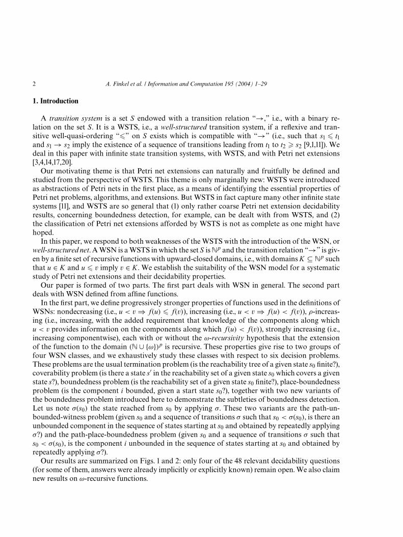
Our results are summarized on Figs. 1 and 2: only four of the 48 relevant decidability questions(for some of them, answers were already implicitly or explicitly known) remain open. We also claimnew results on ω-recursive functions.

A. Finkel et al. / Information and Computation 195 (2004) 1–29 3

Fig. 1. Abbreviations.

Fig. 2. Decidability (D) or undecidability (U) for well-structured nets.

We single out, from the first part of our paper, the following results:

• Coverability forω-WSN, i.e., WSN whose functions satisfy theω-recursivity hypothesis, is showndecidable, while coverability is shownundecidable for ourmost restrictiveWSNclass (i.e., strong-ly increasing WSN) in the absence of the ω-recursivity hypothesis.

• The decidability status of the four boundedness problems for WSN is resolved. This provablyseparates three of our WSN classes, and the fourth class is distinguished from the others whenviewed as a ω-WSN class.

• Boundedness is shown decidable for increasing WSN but undecidable for ω-WSN.• Path-unbounded-witness is shown decidable for �-increasing WSN but undecidable for increas-

ing WSN.• Path-place-boundedness, known to be decidable for reset Petri nets (and for transfer Petri nets),

is shown undecidable for strongly increasing WSN and for ω-WSN.• Place-boundedness is shown decidable for strongly increasingω-WSN. This is proved by showing

that the coverability tree algorithm of Karp and Miller [10,15,16,18] still applies when the exactcomputation of the limit of an infinite repetitive sequence is replaced by the computation of agood enough approximation. Yet, the place-boundedness is shown undecidable for both stronglyincreasing WSN and �-increasing ω-WSN.

In the second part of our paper, we specialize our study to affine WSN, i.e., to WSN definedfrom affine functions. We do this because testing for nontrivial properties of general recursive


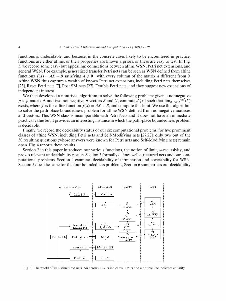
functions is undecidable, and because, in the concrete cases likely to be encountered in practice,functions are either affine, or their properties are known a priori, or these are easy to test. In Fig.3, we record some easy (but appealing) connections between affine WSN, Petri net extensions, andgeneral WSN. For example, generalized transfer Petri nets can be seen as WSN defined from affinefunctions f(X) = AX + B satisfying A � 0 with every column of the matrix A different from 0.Affine WSN thus capture a wealth of known Petri net extensions, including Petri nets themselves[23], Reset Petri nets [7], Post SM nets [27], Double Petri nets, and they suggest new extensions ofindependent interest.

We then developed a nontrivial algorithm to solve the following problem: given a nonnegativep × p-matrix A and two nonnegative p-vectors B and X , compute d � 1 such that limn→ω f nd (X)

exists, where f is the affine function f(X) = AX + B, and compute this limit. We use this algorithmto solve the path-place-boundedness problem for affine WSN defined from nonnegative matricesand vectors. This WSN class is incomparable with Petri Nets and it does not have an immediatepractical value but it provides an interesting instance in which the path-place boundedness problemis decidable.

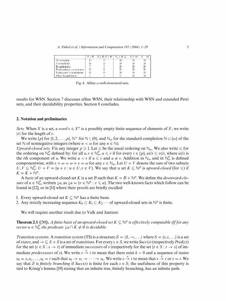
Finally, we record the decidability status of our six computational problems, for five prominentclasses of affine WSN, including Petri nets and Self-Modifying nets [27,28]: only two out of the30 resulting questions (whose answers were known for Petri nets and Self-Modifying nets) remainopen. Fig. 4 reports these results.

Section 2 in this paper introduces our various functions, the notion of limit, ω-recursivity, andproves relevant undecidability results. Section 3 formally defines well-structured nets and our com-putational problems. Section 4 examines decidability of termination and coverability for WSN.Section 5 does the same for the four boundedness problems, Section 6 summarizes our decidability

Fig. 3. The world of well-structured nets. An arrow C → D indicates C ⊂ D and a double line indicates equality.


Fig. 4. Affine ω-well-structured nets.

results for WSN. Section 7 discusses affine WSN, their relationship with WSN and extended Petrinets, and their decidability properties. Section 8 concludes.

2. Notation and preliminaries

Sets. When X is a set, a word v ∈ X ∗ is a possibly empty finite sequence of elements of X ; we write|v| for the length of v.

We write [p] for {1, 2, . . . , p}, �+ for � \ {0}, and �ω for the standard completion � ∪ {ω} of theset � of nonnegative integers (where n < ω for any n ∈ �).Upward-closed sets. Fix any integer p � 1. Let � be the usual ordering on �ω. We also write � forthe ordering on �

pω defined by: for all u, v ∈ �

pω, u � v if for every i ∈ [p], u(i) � v(i), where u(i) is

the ith component of u. We write u < v if u � v and u /= v. Addition in �ω and in �pω is defined

componentwise, with x + ω = ω + x = ω for any x ∈ �ω. Let U + V denote the sum of two subsetsU , V ⊆ �

pω: U + V = {u+ v : u ∈ U , v ∈ V }. We say that a set K ⊆ �p is upward-closed (for �) if

K = K + �p .A basis of an upward-closed set K is a set B such that K = B + �p . We define the downward-clo-

sure of u ∈ �pω, written ↓u, as ↓u = {v ∈ �p : v � u}. The two well-known facts which follow can be

found in [12], or in [11] where their proofs are briefly recalled:

1. Every upward-closed set K ⊆ �p has a finite basis.2. Any strictly increasing sequence K0 ⊂ K1 ⊂ K2 · · · of upward-closed sets in �p is finite.

We will require another result due to Valk and Jantzen:

Theorem 2.1 ([30]). A finite basis of an upward-closed set K ⊆ �p is effectively computable iff for anyvector u ∈ �

pω the predicate ↓u ∩ K /= ∅ is decidable.

Transition systems.A transition system (TS) is a structure S = 〈S ,→, . . .〉where S = {s, t, . . .} is a setof states, and→⊆ S × S is a set of transitions. For every s ∈ S , we write Succ(s) (respectively Pred(s))for the set {t ∈ S : s → t} of immediate successors of s (respectively for the set {t ∈ S : t → s} of im-mediate predecessors of s). We write s

+→ t to mean that there exist k > 0 and a sequence of statess0 = s, s1, . . . , sk = t such that s0 → s1 → · · · → sk . We write s

∗→ t to mean that s+→ t or s = t. We

say that S is finitely branching if Succ(s) is finite for each s ∈ S; the usefulness of this property istied to König’s lemma [19] stating that an infinite tree, finitely branching, has an infinite path.


Reachability. A state t of a TS S is reachable from a state s if s∗→ t.

• The reachability set of S from s0 is denoted RS(S , s0) and is defined as the set of states reachablefrom s0.

• The reachability tree RT(S , s0) of S with the initial state s0 is a directed unordered tree wherenodes are labelled by the states of S . The root node is labelled by s0. A node labelled by s has ason labelled by t iff t ∈ Succ(s). Moreover, any two different sons of a node must have differentlabels.

Orders and limits. Consider an infinite nondecreasing sequence (un)n� 1 of natural numbers. Thissequence is bounded if there exists v ∈ � such that un � v holds for every n ∈ �. We define

limn→ω

un ={ω if (un)n� 1 is not bounded,max{un : n � 1} otherwise.

Now consider a nondecreasing infinite sequence (un)n� 1 of p-tuples un ∈ �p . We also define:

limn→ω

un =(

limn→ω

un(1), limn→ω

un(2), . . . , limn→ω

un(p)).

For our purpose, we shall need the following orders: for any nonempty subset Q ⊆ [p], let <Q

be the strict order relation, called Q-strict order, defined on �pω by:

u <Q v if (u � v) and (∀i ∈ Q, [u(i) < v(i)]).Note that u <Q v implies u <Q′ v for any ∅ /= Q′ ⊆ Q.

The Q-strict order relation is strictly contained in the usual order <. It is well-known that theordering < on �

pω is a well-ordering [6]: for any infinite sequence u0, u1, . . . ∈ �

pω, there exist two

indices i < j with ui � uj . The Q-strict orders (for all Q’s) can be used to refine the latter statement:

Lemma 2.2. For any infinite sequence u0 < u1 < u2 . . . in �pω, there exists a nonempty maximal (w.r.t.

⊆) set Q ⊆ [p] such that there is an infinite subsequence ui0 <Q ui1 <Q ui2 . . . ( with i0 < i1 < i2 . . .).

Proof. Let u0 < u1 < u2 . . . be an infinite sequence in �pω. Recall that any increasing sequence n0 �

n1 � n2 . . . in �ω either is stationary (i.e., there exists an integer k such that nk = nl,∀l � k) or tendstoω. As the sequence (un)n� 0 takes an infinity of values, not all non-decreasing sequences (un(i))n� 0(∀i ∈ [p]), can be stationary. Therefore, we let Q be the (non empty) set of i such that (un(i))n� 0 isnon stationary. �

2.1. Transitions as functions

Throughout this paper, we shall consider transition systems whose sets of states are subsetsof �p , for some p in �. Transitions are considered as recursive functions from �p to �p . Thus,transition functions are not necessarily total. Consider a function f : X → Y . We write Dom f for{x ∈ X | f(x) is defined}. We adopt the convention that we compose functions from right to left, i.e.,


gf(x) = g(f(x)). The notion of growth signature will help us define classes of functions which willillustrate the subtleties of the boundedness question:

Growth signature. The growth signature of an arbitrary function f : �p → �p is the function �f

defined as follows:

�f : {Q ⊆ [p] : Q /= ∅} −→ 2{Q⊆[p]:Q /=∅}

Q �−→ {Q′ ⊆ [p] : ∀u, v ∈ Dom f , [u <Q v �⇒ f(u) <Q′ f(v)]}.Thus theknowledge thatQ′ ∈�f (Q)provides the information that for anyu, v ∈Dom f ,f(u)<Q′ f(v)whenever u <Q v.Types of functions. A function f : �p → �p is

(type 1) nondecreasing if u < v ⇒ f(u) � f(v) for all u, v ∈ Dom f ,(type 2) increasing if u < v ⇒ f(u) < f(v) for all u, v ∈ Dom f ,(type 3) �-increasing if �f (Q) /= ∅ for all nonempty Q ⊆ [p],(type 4) strongly increasing if Q ∈ �f (Q) for all nonempty Q ⊆ [p].

Intuition. A function is strongly increasing if whenever u, v ∈ Dom f and u <Q v, it is guaranteedthat f(u) <Q f(v). The function is only �-increasing1 if the guarantee is only that f(u) <Q′ f(v)for the non-empty sets found in �f (Q); these Q′ may be incomparable with Q. Yet weaker, theincreasing condition only offers the guarantee that f(u) <Q′ f(v) for some Q′, but the latter Q′ maydepend on the particular choice of u and v. Observe that there exist increasing functions that arenot �-increasing. Indeed, the total (hence upward-closed) increasing function f : �2 → �2 givenby

f(i, j) =

(0, 0) if i = j = 0,(i, i − 1) if j = 0 and i is odd,(i − 1, i) if j = 0 and i > 0 is even,(i + 1, i + j) if j > 0

is not �-increasing (this is because, for each n > 0, (2n, 0) <{1} (2n+ 1, 0) <{1} (2n+ 2, 0) and apply-ing f to these pairs yields (2n− 1, 2n) <{1} (2n+ 1, 2n) <{2} (2n+ 1, 2n+ 2), but ¬((2n+ 1, 2n) <{1}(2n+ 1, 2n+ 2)) and ¬((2n− 1, 2n) <{2} (2n+ 1, 2n)), so that no nonempty set R ⊆ {1, 2} fulfills thecondition that, for each u <{1} v with (u, v) in � × �, f(u) <R f(v)).

Proposition 2.3. Let f and g be two functions from �p to �p .

(1) If f and g are of type t above, 1 � t � 4, then gf is again of type t.

(2) If f is nondecreasing and both f and g have upward-closed domains, then the domain of gf isupward-closed.

1 The name �-increasing was given to these functions because the letter � resembles the shape of a path in a finite graphwhich ends in a cycle; see Theorem 5.3.


(3) If f and g are recursive, then gf is recursive.(4) If f is of type t, 1 � t � 4, then f is of type s,∀1 � s � t.

Proof. Straightforward. We nonetheless argue (1) for the case of �-increasing functions. Let f andg be �-increasing functions. Consider ∅ /= Q ⊆ [p]. Pick u, v ∈ Dom gf . Then u, v ∈ Dom f andf(u), f(v) ∈ Dom g. Hence by the �-increasing properties of f and g,

u <Q v �⇒ f(u) <Q′ f(v) �⇒ g(f(u)) <Q′′ g(f(v)),

where Q′ is any nonempty set in �f (Q) and where Q′′ is any nonempty set in �f (Q′). Hence for any

Q, �gf (Q) /= ∅. �

Extension of a nondecreasing function with upward-closed domain.The extension f : �

pω → �

pω of a nondecreasing function f : �p → �p with upward-closed

domain is defined by setting Dom f = Dom f + �pω and, for any v ∈ Dom f :

f (v) = limn→ω

f(vn),

where (vn)n� 0 is any infinite nondecreasing sequence such that v = limn→ω vn. This definition iscorrect because since f is nondecreasing, (f(vn))n� 0 is also a nondecreasing sequence and it admitsa limit in �

pω; moreover for every v ∈ �

pω, there exists an infinite nondecreasing sequence (vn)n�0,

vn ∈ �p such that v = limn→ω vn (in fact, there are an infinite number of sequences having v as limit).Finally, the evaluation of f (v) does not depend on the choice of the sequence (vn)n� 0: given twoinfinite nondecreasing sequences (vn)n� 0 and (v′n)n� 0 such that v = limn→ω vn = limn→ω v′n, onehas that for every n, there exist p , q such that: vn � v′n+p � vn+p+q, hence we also have: for everyn, f(vn) � f(v′n+p ) � f(vn+p+q). Then, limn→ω f(vn) = limn→ω f(v′n). Note that if v ∈ Dom f thenf (v) = f(v).

ω-recursive functions.Let f be a nondecreasing function f : �p → �p with upward-closed domain.We say f is ω-recursive if its extension f is recursive.

We will see in Section 4 that computing f plays a crucial role in deciding the coverability problemand the place-boundedness problem. Here, we note that not all recursive functions f have a com-putable extension f . Indeed, although f is recursive for any fixed nondecreasing recursive functionf : � → � (because f agrees with f on �, and because f (ω) can be hardwired into a machine, i.e.,there exists a machine computing f though we may not know which one), even for a fixed totalrecursive function g : �2 → �2 of type 4, it may not be possible to compute g.

We write TMj for the jth Turing machine (in a classical enumeration) which moreover beginsby writing the integer j on its tape. We say that TMj halts if TMj halts on input j.

Proposition 2.4. There is a strongly increasing total recursive function g : �2 → �2 which is notω-recursive.

Proof . Let g(m, n) = ( m+ |{j � m : TMj halts in at most n steps}|, n). Then g is a strongly increas-ing total recursive function, but g is not computable because


g(m,ω) = g(m− 1,ω)+{(2, 0) if the TMm halts,(1, 0) otherwise. �

The rest of the section studies the impact of the properties of f on the decidability properties of f .Consider adapting in the natural way the nondecreasing, increasing, and strongly increasing

properties to the case of functions f : �p → � for p > 1. Then, increasing and strongly increasingbecome synonymous properties. Furthermore, as for any u in �

pω having at least one component

equal to ω, we must have f (u) = ω, the extension f of any increasing total recursive functionf : �p → � is recursive. On the other hand, projecting onto its first component the function g usedin proving Proposition 2.4 yields a nondecreasing total recursive function g′ : �2 → � that is notω-recursive.

Returning to nondecreasing total recursive functions f : � → �, whose extensions f are recur-sive as we have seen, we might hope to be able to compute the description of a Turing machinecomputing f , given one computing a nondecreasing total f (this is clearly possible when f isincreasing). The next proposition shows that this is impossible. Let NDEC be the set of Turing ma-chines m computing a nondecreasing total recursive function fm : � → �, and let NDECω ⊂ NDEC

comprise those m for which fm(ω) = ω. Now assume to the contrary, that there is a total recursivefunction g such that g(m) is a machine computing f m whenever m ∈ NDEC . Let L be the languageof all m such that the machine g(m) halts on ω and outputs “ω.” Then L is a recursively enumerablelanguage such that L ∩ NDEC = NDECω, which contradicts the following:

Proposition 2.5. Any language L such that

L ∩ NDEC = NDECω

is not recursively enumerable.

Proof. Consider such an L. Note that L is not necessarily an index set so that Rice’s theorem (forrecursively enumerable index sets) does not apply. Consider for each m the Turing machine Mϕ(m)

computing the function fϕ(m) : � → � defined as

fϕ(m)(n) ={t if the TMm halts in exactly t steps and t < n,n otherwise.

Note thatϕ(m) ∈ NDEC for everym. Now theTMm does not halt iff f ϕ(m)(ω) = ω iffϕ(m) ∈ NDECω

iff ϕ(m) ∈ L ∩ NDEC iff ϕ(m) ∈ L. Hence, the recursive map ϕ is a many-one reduction fromthe complement of the halting problem to L, proving that the latter is not recursivelyenumerable. �

2.2. Transitions as affine functions

An affine2 function f : �p → �p is given by f(X) = AX + B for some A = (Ai,j) ∈ �p×p andB ∈ �p and a recursive definition domain Dom f ⊆ {X ∈ �p : AX + B � 0}.

2 We restrict the usual sense of affine functions. In our context, all affine functions have a non negative linear part.


We allowDom f to differ from {X ∈ �p : AX + B � 0}, to be able to simulate transitions of Petrinets. For instance, suppose that, in a Petri net with p places, the transition t only tests whether thereis a token in place 1. This transition is the identity function t(X) = X (hence A = Id and B = 0) andt(X) � 0 for everyX ∈ �p . Yet its definition domain isDom t = �+ × �p−1 and it is not equal to �p .

We denote by Aj the jth column of the matrix A, for any j in [p]. We write A � 0 to mean thatAi,j � 0, for all i, j and A � Id to mean that for all i,Aii � 1 and A � 0.

The following holds for every affine function f defined by f(X) = AX + B:

1. f is nondecreasing,2. f is increasing iff f is �-increasing iff Aj /= 0, for every j in [p],3. f is strongly increasing iff A � Id .

Hence, given an affine function f bywayof its definingmatrixA and vectorB, it is straightforwardto determine its “increasing” property. Moreover, belonging to the set {X ∈ �p : AX + B � 0} iseasily tested, and it is easy to see that this set is upward-closed whenever f is nondecreasing (A � 0).

The composition of two affine functions is affine and every affine function is recursive. Further-more, the extension of a nondecreasing affine function f is recursive as the extension can also bedefined by its affine form AX + B on X ∈ �

pω with the usual conventions 0ω = 0 and mω = ω, for

all m ∈ � such that m > 0.

3. Well-structured nets

We recall [11] that awell-structured transition system (WSTS) is a transition system S = 〈D,→, �〉equipped with a reflexive and transitive relation � ⊆ D × D fulfilling the following two conditions:

(1) well-quasi-ordering: for any infinite sequence s0, s1, . . . ∈ D, there exist two indices i < j withsi � sj .

(2) compatibility: � is (upward) compatible with→, i.e., for any s1 � t1 and transition s1 → s2, thereexists t2 such that t1

∗→ t2 and s2 � t2.

Well-structured nets. A well-structured net (WSN) is a triple S = 〈�p , F , �〉 for some p , where F isa finite set of nondecreasing recursive functions defined on upward-closed subsets of �p .

Intuitively, an ω-well-structured net is a generalization of a WSN defined on �pω. ω-Well-struc-

tured nets. A ω-well-structured net (ω-WSN) is a triple S = 〈�pω, F , �〉 for some p , where F is a finite

set of nondecreasing recursive functions defined on upward-closed subsets of �pω such that for every

function f ∈ F , we have f = fNf where fNf : Nf → Nf is the restriction of f on Nf .A WSN S = 〈�p , F , �〉 or a ω-WSN S = 〈�p

ω, F , �〉 are, respectively,

• increasing if every function in F is increasing,• �-increasing if every function f ∈ F is �-increasing and an algorithm which computes the growth

signature of f is given,• strongly increasing if every function in F is strongly increasing.


Note that a WSN S = 〈�p , F , �〉 gives rise to the WSTS 〈�p ,F→, �〉, where s

F−→t for (s, t) ∈�p × �p is defined to mean that f(s) = t for some f ∈ F . Therefore, we use for S all notions de-

fined for 〈�p ,F→, �〉 (reachability...). In the context of a WSN, a place is an integer; we can speak of

the boundedness of a place: given S and an initial state s0, the place i is bounded if there exists k ∈ �

such that for each s ∈ RS(S , s0), s(i) � k . Note also that everyWSN is finitely branching, because F isfinite.

Remark 3.1. Every Petri netN with p place is a WSN S = 〈�p , F , �〉 such that every function (calledtransition) t ∈ F may be written as t(X) = X + vt , where vt is an integer vector of dimension p . ResetPetri nets are extended Petri nets in which a transition may clear (reset) a place. Formally, a reset Pe-tri net N with p places is a WSN such that every function t in F is an affine function t(X) = AtX + vtin which the matrix (of integers) At satisfies Id � At � 0, where Id and 0 are the identity and thenull matrices respectively, and inequality is taken componentwise.

Let S = 〈�pω, F , �〉 a ω-WSN, s1, s2 ∈ �

pω and � = fkfk−1 . . . f1, with f1, ..., fk ∈ F . We write s1

�−→s2

to mean that there exist t1, ..., tk+1 such that s1 = t1f1−→t2

f2−→t3 → · · · fk−→tk+1 = s2.Given a state so in �p and � = fkfk−1 . . . f1, with f1, ..., fk ∈ F , we define RS(S , s0, �) = {s ∈

�p | s0 �n2−→ s, n ∈ �, 2 prefix of �}.

Proposition 3.2 ([9]). Let S = 〈�p , F , �〉 be a WSN, s1 and s2 two states in �p , and � a finite sequencesuch that s1

�−→s2 and s1 � s2. Then there is a sequence of states (sn)n� 1 such that for all n, sn�−→sn+1

and sn � sn+1.

Problems. We will consider the following computational problems, where in each case, a WSNS = 〈�p , F , �〉 or a ω-WSN S = 〈�p

ω, F , �〉 is given as part of the input:

1. Termination. Given a state s0 in �p , is the reachability tree RT(S , s0) finite?2. Coverability. Given states s0 and s in �p , does there exist a state s′ in RS(S , s0) which covers s, i.e.,

which satisfies s � s′?3. Boundedness. Given a state s0 in �p , is the reachability set RS(S , s0) finite?4. Path-unbounded-witness. This problem is not a decision problem, but rather a search problem in

the sense of [22]: given a state s0 in �p and a finite non empty sequence � such that s0�−→�(s0) and

s0 < �(s0), determine if there is an unbounded place inRS(S , �, s0) (i.e., a place i satisfying ∀k ∈ �,∃s ∈ RS(S , �, s0) such that s(i) � k) and if so identify3 at least one such an unbounded place i.

5. Path-place-boundedness: Given a state s0 in �p , a sequence � such that s0�−→�(s0) and s0 < �(s0),

and a place i, is the place i bounded in RS(S , �, s0) (i.e., does there exist k ∈ � such that s(i) � k ,∀s ∈ RS(S , �, s0))?

6. Place-boundedness: Given an initial state s0 and a place i, is i bounded?

3 Although this problem is not a decision problem, we say that the problem is decidable if there exists a Turing machinewhich solves it (and always halts).


In this list, we have introduced two new problems related to the boundedness problem. ThePath-place-boundedness can be seen as the place-boundedness problem restricted to a particularpath of the reachability tree. It may be decidable when the boundedness problem is not (e.g.reset Petri Nets [7]). Note that decidability of the path-place-boundedness problem implies de-cidability of the path-unbounded-witness problem. As we show later, the reverse implication isfalse.

We do not mention the usual Reachability problem (given two states s and s′, does s∗→ s′

hold?), as it is irrelevant to our paper, being undecidable in all the eight Petri Net extensions weshall study (cf. Fig. 1).

4. When are termination and coverability decidable?

For every state s we denote by ↑s the set {t ∈ D : t � s}.

Theorem 4.1. Termination is decidable for well-structured nets.

Proof. Let S = 〈�p , F , �〉 be a WSN. If s1f−→s2 for a function f ∈ F and s1 � t1, then because

f is nondecreasing and Dom f = ↑Dom f , we have t1f−→t2 and s2 � t2. This property and the

recursivity of f allow us to apply Theorem 4.6 from [11] and then to decide termination. �

Theorem 4.2. Coverability is decidable 4 for ω-well-structured nets.

Proof. We will show that it is possible to compute a finite basis of ↑Pred(↑s) for any s ∈ �p . Thenby using Theorem 3.6 from [11], we will conclude that coverability is decidable. Fix s ∈ �p and writePredf (↑s) for {t ∈ �p | f(t) � s}. We have:

↑Pred(↑s) =↑⋃f∈F

Predf (↑s) =⋃f∈F

↑Predf (↑s) =⋃f∈F

Predf (↑s),

where the rightmost equality uses the fact that ↑Predf (↑s) = Predf (↑s), which holds becauseDom f = ↑Dom f and f is nondecreasing, for every f ∈ F . Because F is finite, it suffices to beable to compute a finite basis of Predf (↑s) for f ∈ F . By Theorem 2.1, namely the Valk and Jantzenresult, a finite basis of Predf (↑s) is computable iff the predicate ↓t ∩ Predf (↑s) /= ∅ is computablefor all t ∈ �

pω. And this holds because

↓ t ∩ Predf (↑s) /= ∅ iff (∃t′ ∈ �p , t′ � t)[f(t′) � s] iff f (t) � s,

where the left to right implication in the second “iff”relies on the non decreasing property of f .Now the inequality f (t) � s can be checked because f is recursive. �

4 Such a statement means: there is a TM deciding the coverability problem, given the premise that the input WSN isan ω-WSN.


The computability of f is a hypothesis needed to decide coverability, since we have as a coun-terpart to Theorem 4.2 that our strongly increasing WSNs have an undecidable coverability whenthis hypothesis is absent:

Theorem 4.3. The coverability problem for strongly increasing well-structured nets is undecidable.5

Proof. Consider the family {fj : �2 → �2} of strongly increasing recursive functions

fj(n, k) ={(n, 0) if k = 0 and TMj runs for more than n steps(n, n+ k) otherwise

and the strongly increasing function g : �2 → �2 defined by g(n, k) = (n+ 1, k). The strongly in-creasing WSN Sj = 〈�2, {fj , g}, �〉 with initial state (0, 0) has the property that the state (1, 1) iscoverable iff the TMj halts. Hence there is no Turing machine which correctly determines cover-ability and halts whenever its input is a strongly increasing WSN. �

5. When are boundedness problems decidable?

5.1. The boundedness problem

An increasing WSN verifies the property that if s1 → s2 and t1 > s1, then there exists t2 such thatt1 → t2 with t2 > s2, while we can only conclude t2 � s2 in the case of a WSN. Boundedness forincreasing WSNs can thus be decided by searching for a sequence s0

∗→ s1�→ s2 with s1 < s2. Then,

� can be iterated to produce an increasing sequence of reachable states s0∗→ s1

�→ s2�→ s3 . . . with

s1 < s2 < s3 . . ., and the system is unbounded. Because any WSN by definition has a recursive Succ(i.e., Succ(s) is computable, for every s in �p ), Theorem 4.11 from [11] yields:

Theorem 5.1. Boundedness is decidable for increasing well-structured nets.

We note further that Theorem 5.1 is tight. If we omit the “increasing” property from the hypoth-esis of Theorem 5.1, and yet add the “ω-recursivity” property, the boundedness problem becomesundecidable:

Theorem 5.2. Boundedness is undecidable for ω-well-structured nets.

Proof. Boundedness is undecidable for reset Petri nets [7], which are affine WSNs and every affineWSN is a ω-WSN (see Section 2.2). �

5 The precise technical meaning of this statement is that there is no Turing machine which correctly decides whethersome state in RS(S , s0) covers s, and halts, whenever its input S is indeed a strongly increasing WSN (with its definingfunctions given by Turing machines) together with s0 and s.


5.2. The path-unbounded-witness problem

In this section, we show how to detect at least one unbounded place in some unbounded WSNs.Indeed we show the problem decidable for �-increasing WSNs. This decidability result provablydoes not extend to increasing WSNs, as we also prove in this section.

Theorem 5.3. The path-unbounded-witness problem is decidable for �-increasing WSN.

Proof. Consider a �-increasing WSN S = 〈�p , F , �〉. Consider the edge-labelled graph

G = ({Q ⊆ [p] : Q /= ∅}, {(Q, f ,Q′) : Q′ ∈ �f (Q)}),where �f is the (computable) growth signature of f . Consider any non empty finite path in thisgraph from a node Q to a node Q′. Let f1, f2, . . . , fk be the sequence of edge labels encounteredalong the path. A straigthforward induction on k proves that

∀u, v ∈ Dom fkfk−1 · · · f1, [u <Q v �⇒ fkfk−1 · · · f1(u) <Q′ fkfk−1 · · · f1(v)]. (1)

Now let a state s0 and a sequence � = f1f2 · · · fk be given such that s0 < �(s0). Let Q be thenonempty set such that s0 <Q �(s0). Our goal is to determine a place along which iterating � froms0, (which is always possible because Dom � is upward-closed), grows unbounded. Because eachf ∈ F is �-increasing, each node in G has at least one outgoing edge labelled f . Because G is finite,there exists a computable finite path � in G with the following properties:

• � starts at node Q,• � visits nodes Q = Q0,Q1,Q2, . . . ,Qk·j ,Qk·j+1, . . . ,Qk·l for some j, such that 1 � j < l and Qk·j =

Qk·l(= Q′),• � traverses the edges labelled f1, f2, . . . , fk , f1, f2, . . . , fk , f1, f2, . . . , fk , f1, . . . , fk .

Applying (1) inductively shows that �i(s0) <Qk·i �i+1(s0) for 1 � i < l.

In particular,

s0 � �j(s0) � �l−1(s0) <Q′ �l(s0).

Write d = l− j. Because the last k · d steps of � form a cycle c around Q′, this cycle can be repeatedarbitrarily often to extend �. Since the sequence of edge labels forming c spells �d , each extensionof � by c reflects the effect of further applying �d . Applying (1) again,

�l(s0) � �l+d−1(s0)

<Q′ �l+d (s0)

� �l+2·d−1(s0)

<Q′ �l+2·d (s0)� · · ·<Q′ �l+m·d (s0)� · · ·


This implies that all the places in the non-empty set Q′ grow unbounded when � is iterated from s0.Hence any place in Q′ is a satisfactory answer. �

Theorem 5.3 is tight. It provably extends neither to the guaranteed identification of at least oneunbounded place in increasing well-structured nets, as we now show, nor to the decidability ofpath-place-boundedness in �-increasing WSN, as we will show in the next section.

Theorem 5.4. The path-unbounded-witness problem is undecidable for increasing well-structured nets.

Proof. For each m, we define f ′m : �2 → �2 by

f ′m(k , n) =

{(k , n+ 1) if the TMm halts in at most k − 1 steps(k + 1, n) otherwise.

Every f ′m is total (hence upward-closed), recursive, and increasing.

Now, from any initial state (k , n) ∈ �2, the increasing WSN Sm = 〈�2, {f ′m}, �〉 possesses one and

only one unbounded place, which is the second place iff the TMm halts. Suppose to the contrary thatthere is a TM M which solves the path-unbounded-witness problem. On input s1 = (0, 0), � = f ′

m,and s2 = (1, 0), M will necessarily come up with the unique unbounded place resulting from the iter-ation of f ′

m from s1. This place is the second place if TMm halts, and the first place otherwise, whichmeans that M solves the halting problem. Hence no such M exists, and so path-unbounded-witnessproblem is undecidable. �

5.3. The path-place-boundedness problem

Theorem 5.5. Path-place-boundedness is undecidable for strongly increasing well-structured nets andfor ω-well-structured nets.

Proof.

• Consider the strongly increasing WSN Sj = 〈�2, {fj , g}, �〉 from the proof of Theorem 4.3, withinitial state (0, 0) and the sequence � = gfj . Then, place 2 is unbounded along the infinite path(0, 0)

�→ �→ �→ ... if and only if TMj halts.• Consider the family of functions gj : � → � defined by

gj(n) ={n if TMj halts in at most n stepsn+ 1 otherwise.

For every j � 1, the function gj is nondecreasing, total, and ω-recursive (gj(ω) = ω). Let

Tj = 〈�, {gj}, �〉with initial state 0. The only place is bounded along the infinite path 0gj→ ...

gj→ ...

if and only if the TMj halts. �

The following proposition justifies our interest in the path-place boundedness problem. Althoughboundedness in undecidable for Reset Petri nets [7], path-place boundedness is decidable.


Proposition 5.6. Path-place-boundedness is decidable for reset Petri nets.

Proof . Given a reset Petri net N with p places, a marking m, a place i and a sequence � of transi-tions such that m

�→ m1 with m < m1. By monotonicity, (� is non-decreasing), the sequence � maybe infinitely repeated; let us write the infinite path m

�→ m1�→ m2

�→ · · ·.Let us write � = fkfk−1...f1. Because each affine function fi(X) = AiX + vi satisfies 0 � Ai � Id

and vi is a vector of integers, we deduce that there exist A� and v� such that � is the affine function�(X) = A�X + v� with still 0 � A� � Id and v� a vector of integers (where A� is computable fromthe Ai’s and v� from the vi’s and Ai’s).

For every n and 1 � j � p , we have: if � does not contain any reset operation on j (i.e.,A�(j, j) = 1)then mn(j) = m(j)+ nv�(j); moreover, if � contains a reset operation on place j, then the sequence(mn(j))n� 1 is stationary and for every n, 2 � n, mn(j) = m1(j) and hence place j is bounded alongthe path m

�→ m1�→ m2

�→ · · ·.We will now prove that i is unbounded along the infinite path m

�→ m1�→ m2

�→ · · · iff m1 � m2and m1(i) < m2(i).

(1) If i is unbounded along the infinite path m�→ m1

�→ m2�→ · · ·, then � cannot contain any reset

operation on place i (hence A�(i, i) = 1), v� must be positive (otherwise the path would be finite);hence, we obtain that for every n, 1 � n, mn � mn+1. Moreover, we can find two integers r andk such that: 1 � r, 1 � k , mr � mr+k , and mr(i) < mr+k(i).Hence, frommr(i) < mr+k(i) and 0 < k , we obtain 0 < v�(i). Hence, we also have:m1(i) < m2(i).

(2) Let us prove that if m1 � m2 and m1(i) < m2(i) then i is unbounded along the infinite pathm

�→ m1�→ m2

�→ · · ·. First, by monotonicity, (� is non-decreasing), the path can be infinite-ly continued and then 0 � v� . Because m1(i) < m2(i), the sequence � cannot contain any re-set operation on place i and then 1 � v�(i). From mn(i) = m(i)+ nv�(i), we obtain that mn(i)

goes to infinity when n goes to infinity. Hence, the place i is not bounded on the infinite pathm

�→ m1�→ m2

�→ · · ·. �

5.4. The place-boundedness problem

Let us recall the construction of the coverability tree of a Petri net, which is used to solve theplace-boundedness problem. The strategy of the construction is to develop every path of the reach-ability tree until one meets two markings m and m′ such that m0

∗−→ m�−→ m′ with m <Q m′ and

Q the maximal nonempty subset of places for this property. When one meets two such markings mand m′, one replaces m′ by the limit of the infinite increasing sequence of markings obtained fromm by iterating �. This limit is exactly and effectively computable for Petri nets (and for transfer andreset Petri nets as well):

limn→ω

(�n(m))(i) ={ω if i ∈ Q

m(i) if i /∈ Q.

Then one continues using the same strategy with all transitions extended from �p to �pω. Termina-

tion is guaranteed because � is still a well-ordering on �pω.


To apply the above strategy to construct a coverability tree for a WSN, it is first necessary tobe able to effectively extend functions to �

pω. This means that functions have to be ω-recursive.

Furthermore, the extension f of any nondecreasing function f is nondecreasing, but any type-iproperty of f may not be preserved on f . In particular, strongly increasing functions extend-ed to �

pω may no longer be increasing (for example, when f is defined as f(m, n) = (m,m+ n),

f(ω, 0) = f(ω, 1)).Moreover, either limn→ω �n(u) must be computable (but this is not true for nondecreasing ω-re-

cursive functions), or a good enough approximation lof limn→ω �n(u)must be computable such thatu < l � limn→ω �n(u) and l has at least one more ω-component than u, for every infinite increasingsequence (�n(u))n� 1.

Let ω-max be the following function which takes two elements s1 and s2 in �pω and returns an

element in �pω, defined by:

function ω-max(s1, s2): returns s : �pω

s ← s2for each i such thats1(i) < s2(i) and s2(i) /= ω dos(i) ← ω;

We will only apply this function to pairs of states (s1, s2) satisfying s1 � s2. Note that in gen-eral, ω-max can satisfy ω-max(u, �(u)) < limn→ω �n(u), for example when f(m, n) = (m+ n, n+1) and u = (0, 0), in which case f(u) = (0, 1) and ω-max(u, f(u)) = (0,ω), while limn→ω f n(u) =(ω,ω).

Nevertheless, any strongly increasing WSN satisfies the interesting property:

Proposition 5.7. Let 〈�p , F , �〉 be a strongly increasing WSN and let u, v be in �pω. If there exist

f1, . . . , fk in F such that u�−→ v for � = f k f k−1 . . . f 1, and there exists a nonempty Q such that

u <Q v, then limn→ω �n(u) � ω-max(u, v) > v, and ω-max(u, v) contains |Q| more ω’s than u.

Proof. As (�n(u))n� 1 is a nondecreasing sequence, limn→ω �n(u) exists. As a composition of stronglyincreasing functions, � is strongly increasing. So u

�−→ v and u <Q v imply �n(u) <Q �n+1(u), forany positive integer n. So for i in Q, limn→ω �n(u)(i) = ω and for i not in Q, we do not know if thislimit is finite or not, but at least we have limn→ω �n(u) � ω-max(u, v) � v. Note that ω-max(u, v)contains |Q| more ω than u. �

It is possible to apply (after a natural generalization which replaces the Petri net transitions byω-recursive functions) the Karp–Miller algorithm (originally designed to compute a coverabilitytree of a Petri net) [18] to the more abstract model, ω-WSNs.

Let S = 〈�pω, F , �〉 be an ω-WSN and s0 an initial state in �

pω. The Karp–Miller tree of S start-

ing at s0, denoted KMT(S , s0), is the tree produced by the following extended Karp–Milleralgorithm. It is a labelled tree consisting of a set of nodes NODES ⊆ � and a set of arcs ARCS⊆ NODES × NODES; each node is labelled with a state from �

pω and each arc is labelled with a

function from F .(We refer to a node as a pair (i, s) to indicate that the node i ∈ � is labelled s ∈ �

pω; we refer

to an arc as a triple (i, f , j) to indicate that (i, j) is an arc labelled f ∈ F .) In the algorithm andlater, we will use the notations (n1, s1)

�−→KMT (n, s), (respectively (n1, s1)∗−→KMT (n, s), respective-


ly (n1, s1)+−→KMT (n, s)) for saying that there is path labelled by � (respectively a possibly empty,

respectively non-empty) path in KMT from node (n1, s1) to the node (n, s).

Karp–Miller_tree (〈�pω, F , �〉 : ω-WSN, s0 : state in �

pω) returns KMT: tree

NODES ← ∅; ARCS ← ∅;UNPROCESSED_NODES ← {(0, s0)}; {* Initial singleton set of unprocessed nodes,each node referred to as “(node number, temporary label)” *}while a node (n, s) is in UNPROCESSED_NODES do

UNPROCESSED_NODES ← UNPROCESSED_NODES \ {(n, s)};for all nodes (ni, si) such that (ni, si)

∗−→KMT (n, s) and si < s dos ← ω-max(si, s);

NODES ← NODES ∪ {(n, s)}; {* Add node and fix label forever *}

if no node (n1, s) exists such that (n1, s)+−→KMT (n, s) then

for each function f ∈ F such that s ∈ Dom f don′ ← new node number;UNPROCESSED_NODES ← UNPROCESSED_NODES ∪ {(n′, f (s))};ARCS ← ARCS ∪ {(n, f , n′)};

KMT ← (NODES ,ARCS);

Before proving that the algorithm terminates on all ω-WSNs, we remark some useful elementaryfacts about the finite paths of the Karp–Miller tree.

Lemma 5.8.LetS=〈�pω, F , �〉beanω-WSN, s0 an initial state in�

pω andKMT(S , s0) theKarp–Miller

tree of (S , s0). We have:

• If (0, s0)∗−→KMT (n1, s)

∗−→KMT (n2, s) then the node n2 has no successor(along a branch of the KMT, the same state cannot appear more than twice).

• if (n, s)�−→KMT (n′, s′) then �(s) � s′.

• if (n, s)∗−→KMT (n′, s′) and s < s′ then s′ has at least one ω more than s.

Proposition 5.9. The Karp–Miller tree algorithm terminates when it is applied to an ω-WSN.

Proof. Suppose that the Karp–Miller tree algorithm does not terminate and so KMT is infinite.Because the set of functions is finite, the infinite tree KMT is finitely branching and there is aninfinite branch in KMT:

(0, s0) −→KMT (n1, s1) −→KMT .... −→KMT (nk , sk) −→KMT ...

Because � is a well-ordering on �pω, we may extract an infinite non-decreasing sequence {ski} that

cannot be stationary (by Lemma 5.8).So we may also choose an infinite increasing sequence along this branch:

(nk0 , sk0)∗−→KMT (nk1 , sk1)

∗−→KMT .... with ski < ski+1


We recall that (n, s)∗−→KMT (n′, s′) and s < s′ imply that s′ must contain at least one ω more than

s, by Lemma 5.8.After a finite number (at least p) of such executions, no “new ω” can be inserted. Hence, for every

n, skp = skp+n and the sequence (skn)n� 1 is stationary, which produces a contradiction. Hence KMTis finite. �

In the following, we will say “a state s in KMT(S , s0),” for “a state s such that there exists a node(n, s) in KMT(S , s0).”

When the Karp–Miller algorithm is applied to an ω-WSN, it produces a finite tree such thatevery reachable state is smaller than (or equal to) a state in KMT (see Proposition 5.11). But ingeneral, the KMT may very roughly cover the reachability set, in the following sense: some state inthe KMT may be strictly greater than the limit of any infinite sequence of reachable states. Whenthe Karp–Miller algorithm is applied to a strongly increasing ω-WSN, it produces a tree, oftencalled a coverability tree, which finely covers the reachability set: each state in KMT is smallerthan (or equal to) the limit of an infinite sequence of reachable states. The following property ofstrongly increasing functions (with upward-closed domain) is used for proving that the cover isfine.

Lemma 5.10. Let f : �p → �p be any strongly increasing function with upward-closed domain. Let(un)n� 1 be a nondecreasing sequence in Dom f and u its limit in �

pω. There exists a strictly increasing

sequence of natural numbers (ϕ(n))n� 1 such that limn→ω f n(u) = limn→ω f n(uϕ(n)).

Proof. Let us recall that any nondecreasing sequence in �ω either goes to ω, either isstationary. For all m, we define Im as the set of places i such that the nondecreasing sequence(f m(un)(i))n� 1 is non stationary. Let i ∈ Im. Then for all integer n, there exists p > n such thatf m(un)(i) < f m(up)(i). Because f is strongly increasing, f m+1(un)(i) < f m+1(up )(i). Therefore i ∈Im+1. We have shown the sequence (Im)m�1 is nondecreasing (for ⊆), therefore there exist a sub-set I of places and a natural number N such that Im = I for all m � N . These I and N

satisfy:

(1) For i ∈ I and m � N , the sequence (f m(un)(i))n� 1 is non stationary, thus its limit value is ω. Wemay write:∀m � N , ∃7m > 0 such that ∀i ∈ I , ∀n � 7m, we have f m(un)(i) > m.

(2) For i /∈ I and m � N , the sequence (f m(un)(i))n� 1 is stationary. Thus the limit value must bef

m(u)(i). In that case, we may write:

∀m � N , ∃8m > 0 such that ∀i /∈ I , ∀n � 8m, we have f m(un)(i) = fm(u)(i).

For all m � N , we define by induction ϕ(m) as the maximum of Am, Bm, and ϕ(m− 1)+ 1. Wethen have:

(1) For i ∈ I and m � N , f m(uϕ(m))(i) > m.(2) For i /∈ I and m � N , f m(uϕ(m))(i) = f

m(u)(i).

Hence, we have limn→ω fn(u) = limn→ω f n(uϕ(n)). �


Proposition 5.11.For every ω-WSN S = 〈�p

ω, F , �〉 with initial state s0, we have:

1. for every state s ∈ RS(S , s0), there exists a state s′ ∈ KMT(S , s0) such that s � s′,2. If, moreover S is strongly increasing, we have: for every state s ∈ KMT(S , s0), there exists an

infinite non decreasing sequence (sn)n� 1 of reachable states sn ∈ RS(S , s0) such that s �limn→ω sn.

Proof .

1. Let s be a reachable state in RS(S , s0); we will use induction on the length of � with s0�−→

s. When � is the empty word, the statement holds because it is always true that s0 ∈KMT(S , s0).Consider a sequence (in the reachability tree) �f of length k + 1. We define inductively �f = �f .

From s0�−→ s

f−→ f(s) and the induction hypothesis, we deduce that there exists (0, s0)∗−→KMT

(n′, s′) with s′ ∈ �pω and s � s′. Because s � s′ and f is nondecreasing, we obtain f (s) � f (s′).

Now there are two possible cases:

• The node (n′, s′) has no successor. This is necessarily because there exists a path (n1, s′)∗−→KMT

(n′, s′).Because f (s′) exists, the node (n1, s′) has at least one successor (n′′, t) such that: (n1, s′)

f−→KMT

(n′′, t) with f (s′) � t.

• The node (n′, s′) has at least one successor then there is an arc labelled f : (n′, s′) f−→KMT (n′′, t)with f (s′) � t.

In both cases, we have: there exists a state t in KMT such that t � f (s′) � f(s).2. We use induction on the number of times k one has used the function ω-max on a sub-path (in

KMT) from the initial state to state s.

• Let k = 0; suppose that there is a branch (0, s0)∗−→KMT (n, s) such that the function ω-max

has not been used along this branch. Then s is a reachable state and we may write sn = s forevery n.

• Now let k = n+ 1, and consider (0, s0)∗−→KMT (n1, s)

�−→KMT (n2, t) in which the lastapplication (in the Karp–Miller algorithm) of the function ω-max occurred directlybefore n2, whence: t = ω-max(s, �(s)). Then by the induction hypothesis, there exists aninfinite nondecreasing sequence of reachable states (sn)n� 1 such that s � limn→ωsn;and from the algorithm, we may deduce that s <Q �(s) for a maximal non-empty subset Q

of [p].From s <Q �(s), we deduce that the sequence (�n(s))n� 1 is an infinite nondecreasing sequencewhose limit is written l = limn→ω�

n(s). From Proposition 5.7, we have l � t and from Lemma5.10, there exists a function ϕ such that l � limn→ω�

n(sϕ(n)) because s � limn→ωsn. Hence wehave found an infinite nondecreasing sequence of reachable states (�n(sϕ(n)))n� 1 whose limitis greater than t. �


Remark 5.12. From the last proposition, we may prove that for every infinite nondecreasing se-quenceof reachable states (sn)n� 1, there exists a state t in theKarp–Miller tree such that limn→ωsn� t;in general, there is no reason for having: limn→ωsn = t. Moreover, every state t in KMT isnot necessarily the limit of an infinite nondecreasing sequence of reachable states. Hence forstrongly increasing ω-WSN, the Karp–Miller tree does not exactly enjoy the same properties asthose defined for Petri nets. But we still have a strong relation between the Karp–Miller treeand the reachability set: ↓KMT(S , s0) =↓RS(S , s0) where ↓KMT(S , s0) is the downward-closureof the set of states occurring in KMT(S , s0); this is sufficient for deciding the place-boundednessproblem.

We thus obtain:

Theorem 5.13. For a strongly increasing ω-well-structured net 〈�pω, F , �〉, place-boundedness is

decidable.

Proof. From Proposition 5.11, we show that a place i is not bounded in S = 〈�pω, F , �〉with the initial

state s0 iff there is anode (n, t) inKMT(S , s0) such that t(i) = ω. Bydefinition, i is notbounded in (S , s0)means that there exists an infinite sequence of reachable states (tn)n� 1 such that limn→ωtn(i) = ω.Hence, from Proposition 5.11 (1), we obtain that if i is not bounded in (S , s0) then there existst′ ∈ KMT(S , s0) such that t′(i) = ω. Conversely: suppose there is a t ∈ KMT(S , s0) such that t(i) = ω.FromProposition 5.11 (2), there exists an infinite non-decreasing sequence of reachable states (sn)n� 1such that: t � limn→ωsn. Hence, limn→ωsn(i) = ω and i is not bounded in (S , s0). Because the KMTalgorithm terminates (cf. Proposition 5.9) forω-well-structured nets, we conclude that place-bound-edness is decidable. �

Theorem 5.13 is optimal in the following sense:

Theorem 5.14. Place boundedness is undecidable for both strongly increasing well-structured nets andfor �-increasing ω-well-structured nets.

Proof. Undecidability of place-boundedness holds for �-increasing ω-WSN because transferPetri nets [7] are �-increasing ω-WSN and undecidability of place-boundedness holds forthose. For proving the undecidability for strongly increasing WSN, we again use the family{Sj} with initial state (0, 0) as in Theorem 4.3. The place 2 is unbounded if and only if TMj

halts. �

6. Summary

Recall the six problems defined in Section 3. We have shown in Sections 4 and 5 the followingresults:

Theorem 6.1.The decidability status of the six problems defined in Section 3 of this paper, for the eightclasses depicted in Fig. 1, is summarized on Fig. 3.


7. Affine realizations of well-structured nets

7.1. On the difficulty of testing general recursive functions

Given a set F of functions �p → �p prescribed by their respective Turing machines, decidingwhether F gives rise to a WSN is undecidable, a consequence of Rice’s theorem [25] which we stateas Proposition 7.1:

Proposition 7.1. For each type (t) of function chosen from (1) nondecreasing, (2) increasing, (3)�-in-creasing, and (4) strongly increasing, the following languages

(a) {k | the kth TM computes f : � → � of type (t)}(b) {k | the kth TM computes f : � → � of type (t) whose domain is upward-closed}(c) {k | the kth TM computes f : � → � whose domain is upward-closed}

are undecidable.

Nevertheless, in concrete cases, it is generally known or easy to decide in which class the giv-en set of functions lies. In many Petri net extensions, this given set is in fact contained in theset of affine functions. Many connections between affine functions and Petri net extensions areshown in Fig. 2. Section 7.2 describes WSN for which deciding the properties of relevant func-tions is easy. Section 7.4 summarizes the decidability status of problems involving affinefunctions.

7.2. Petri net extensions and affine well-structured nets

In Section 2.2, we discussed the fact that every affine WSN is a ω-WSN.Figs. 3 and 4 locate Petri net extensions within our classes of affine functions. Fig. 3 also locates

the affine classes within our general framework of well-structured nets.The Double Petri nets [7] appearing on Fig. 3 are extended Petri nets in which some arc from a

transition to a place p may double the content of p . Double Petri nets are then affine WSN such thatevery affine function f(X) = AX + B satisfies Id � A � 2Id . Transfer Petri nets [7] are extended Petrinets in which some transitions may transfer the content of a place p to another place p ′. TransferPetri nets are then affine WSN such that every affine function f(X) = AX + B satisfies A � 0 andevery column Aj satisfies :iAij = 1. Generalized Transfer Petri nets may transfer and duplicate, sothat they are affine WSN such that A � 0 and every column Aj is nonnull. Reset Petri nets [2,7] areextended Petri nets in which an arc may clear a place. This class corresponds to affine WSN suchthat every affine function f(X) = AX + B satisfies Id � A � 0.

Many Petri net extensions are thus surprisingly well parametrized by affine functions.

7.3. An algorithm for path-place-boundedness

A nonnegative affine function is an affine function f : �p → �p such that f(X) = AX + B withB � 0.


A nonnegative affine WSN is a WSN such that every function f ∈ F is nonnegative affine.6 Weprove here that path-place-boundedness is decidable for nonnegative affine WSN.

For f a nonnegative affine function and X a nonnegative vector in �p , we prove that the limit off nd (X) for a suitable d is computable.We can determine preciselywhich entries in f nd (X) go to infin-ity and therefore which entries in f nd+r(X).7 go to infinity, for all r such that 0 � r � d − 1. Further-more, we show that this limit is computable by searching a computable graph. Let f(X) = AX + B

be a nonnegative affine function. Note that, for n ∈ �, f n is also a non negative affine function,precisely: f n(X) = AnX + (An−1 + An−2 + · · · + A+ I)B.

Recall that multiplication is extended by 0ω = 0 and xω = ω, ∀x ∈ �ω − {0}. Let’s first remarkthe following:

Lemma 7.2. Let (An)n� 0 be a sequence of non negative matrices having a limit A with possibly ω

coefficients. Let X be any non negative vector. Then limn→ω AnX = AX.

So we may restrict the problem to the study of the sequences (An)n� 0 and (I + A+ · · · + An)n� 0.

Notations. Let A be a matrix. We write A = 0 or A = ω when each coefficient of A is respectively 0or ω. We write Aω for limn→ω An when the limit exists.

Let A = (Ai,j)(i,j)∈[p]×[p] be a matrix with nonnegative integers coefficients. Let us denote An =(A

(n)i,j ) (where the brackets in the exponent are used to avoid confusion with the (i, j)-entry of A

raised to the nth power).We associate to A a directed graphGA whose vertices are 1, . . . , p and whose set of edges is defined

by: there is an edge leaving vertex i and entering vertex j if and only if Ai,j /= 0; then, the coefficientAi,j is called the weight of this edge. For a subgraph C of GA, we shall denote by AC the submatrix(Ai,j)(i,j)∈C×C . We shall need the general decomposition of a non-negative matrix A in term of itsassociate graph GA, as it is usually done in the study of finite homogeneous Markov chains or theproof of Perron-Frobenius theorem (cf. [13], [21], [26]).

A path of length n from a vertex i to a vertex j is a sequence i = i0, i1, . . . , in−1, in = j such that(ik ,ik+1) is an edge inGA, for k=0, 1, . . . , n− 1.Theweightof this path is theproductAi,i1Ai1,i2 . . . Ain−1,j .The path i = i0, i1, . . . , in−1, in = j is called a cycle whenever n /= 0 and i = j. The cycle i = i0, i1, . . . ,in−1, in = i is called a circuit if i0, i1, . . . , in−1 are distinct. The index of imprimitivity of a graph is theg.c.d. of the lengths of all circuits of the graph. When this index of imprimitivity is equal to 1, wesay the graph is primitive. We first recall two properties of this index of imprimitivity:

Lemma 7.3. Let G be a graph whose index of imprimitivity is denoted by d. Let i be a vertex of G.

Then all cycles going through i in G have lengths multiple of d.

6 A nonnegative affine function f : X �→ AX + B in a WSN satisfies A � 0 and B � 0, as f is required to be nonde-creasing.

7 If we denote by L(X) the limit of (f nd (X))n� 0, whenever d > 1, the d sub-sequences (f nd (X))n� 0,(f nd+1(X))n� 0, . . . , (f nd+d−1(X))n� 0 are convergent with respective limits L(X), f(L(X)), . . . , f d−1(L(X)).


Proof. Let i = i0, i1, . . . , in−1, in = i be a cycle of length n going through i. Let us show that n is amultiple of d by induction: If i0, i1, . . . , in−1 are distinct, then this cycle is a circuit and n is a multipleof d by definition. Otherwise, let k , l with 0 � k < l � n be such that ik = il. Take l as small aspossible. So ik , ik+1, . . . , il is a circuit of length l− k , which implies l− k is a multiple of d . Andi0, i1, ik , il+1 . . . , in−1 is a cycle of length n− l+ k < n, thus a multiple of d by induction. �

Lemma 7.4. Let G be a strongly connected graph whose index of imprimitivity is denoted by d. Let ibe a vertex of G. Then d is the g.c.d. of the lengths of all cycles going through i in G.

Proof. Let e be the g.c.d. of the lengths of all cycles going through i in G. Thanks to Lemma 7.3e is a multiple of d . Let j = j0, j1, . . . , jn−1, jn = j be a circuit in G. Let i = i0, i1, . . . , il = j be apath going from i to j and let j = il+1, il+2, . . . , im = i be a path going from j to i in G. Then, i =i0, i1, . . . , il = j0, j1, . . . , jn = il+1, il+2, . . . , im = i and i = i0, i1, . . . , il = il+1, il+2, . . . , im = i are cyclesgoing through i, thus their lengths are multiple of e. thus, the length of the circuit is a multiple of e.This shows d is a multiple of e. �

As we shall see, the asymptotic of the sequence (An)n� 0 may be completely described by thegraph GA. The proof is based on the fact that A(n)

i,j is the sum of the weights of all paths of length n

from i to j.The next two results correspond to particular cases of the final result of this section.

Lemma 7.5. Let C be a strongly connected component of GA whose index of imprimitivity is equalto 1. Then, either C is reduced to a singleton and AC is one of the 1 × 1 matrices (0) or (1), orAωC = ω.

Proof . Recall some facts about primitive strongly connected graphs : We discard the case wherethe graph C has no edge at all, i.e., C is a singleton and AC = (0). Let i, j in C . Note that becauseC is strongly connected there exists a path from i to j (so there exists t such that A

(t)i,j > 0) and

there exists a path from i to j which goes through all vertices of C . Because C is maximal for thisproperty, all paths from i to j in GA are in fact in C . Furthermore, we may find circuits in C withlengths l1,l2,. . ., lk such that g.c.d.(l1, l2, . . . , lk) = 1. With a path of length l0 from i to j crossing allthese circuits, we can build a path in C of length l0 + n1l1 + n2l2 + · · · + nklk , for any non negativeintegers n1, n2, . . . nk . It means there exists a path from i to j of any large enough length, i.e., ∃q ∈ �

such that A(n)i,j > 0 for n > q.

• If A(n)i,i = 1, for sufficiently large integers n, then there is only one circuit in AC with all edges

labelled by 1. So AC is a permutation matrix, which means GAC is a disjoint union of circuits. ButGAC = C is strongly connected and the index of imprimitivity of C is equal to 1, so AC = (1).

• Otherwise, there exists s such that A(s)i,i � 2. Let i, i1, . . . , ir−1, j a path of length r from i to j

and let q be such that A(n)j,j > 0, if n � q. Now, if n � s+ q+ r, we may decompose n as u+

r + ts with u ∈ {q, . . . , q+ s− 1} such that u ≡ n− r modulo s and t >n−q−s−r

s . Then A(n)i,j �

(A(s)i,i )

tAi,i1 . . . Air−1,jA(u)j,j � 2t which shows limn→ω A

(n)i,j = ω. �


Lemma 7.6.LetC be a strongly connected component ofGA with index of imprimitivity equal to c > 1.Let D,E two strongly connected components of GAc

Cand (i, j) ∈ D × E. Then

(Ac)ωi,j =

0 if D /= E

1 if {i} = D = E = {j} and A(c)i,i = 1

ω otherwise.

Proof. Let us first remark that there exists a path of length l from i to j in GAcC

if and only if thereexists a path of length cl from i to j in GA. Let D be a strongly connected component of GAc

Cand i

be a vertex of D. Thanks to Lemma 7.4, the index of imprimitivity of D is the g.c.d. of the lengths ofall cycles in GAc

Cgoing through i, i.e., the quotient by c of the g.c.d. of the lengths of all cycles in GA

going through i. Therefore, it is equal to 1. Let D,E two strongly connected components of GAcC

and(i, j) ∈ D × E. If D /= E, there cannot exist a path from i to j and a path from j to i in GAc

C. Let us

suppose, for example, that i cannot be joined to j by a path in GAcC, which means i cannot be joined

to j by a path of length multiple of c in GA. As all cycles have lengths multiple of c, j cannot bejoined either to i by a path of length multiple of c. So ∀n, A(nc)

i,j = A(nc)j,i = 0. When D = E, we apply

Lemma 7.5 to (A(c)(i,j))(i,j)∈D×D which defines a strongly connected graph with index of imprimitivity

equal to 1. �

The general case: The next theorem explains how to describe the behaviour of the sequence(An)n� 0, without making any assumption of strong connectivity or on the index of imprimitivityof the graph GA associated to the matrix A. We compute the strongly connected components ofGA. Grouping nodes by components, we find a permutation matrix P such that PAP−1 is a triangu-lar-blocks matrix where each diagonal block is irreducible (corresponding to a strongly connectedcomponent of GA). Let d be the l.c.m. of the indices of imprimitivity of all components of GA. Wealready know by the two previous lemma how to compute the limit of the powers of each irreduciblediagonal block of Ad . Let r be the number of strongly connected components of GAd . We partitionthe matrix B = PAdP−1 = (Bi,j)(i,j)∈[r]×[r] such that each block Bi,i corresponds to a strongly con-nected component of GAd . We shall call this component a 0, 1 or ω block according to the nature ofits limit in Lemma 7.5.

We consider the graph GB: vertices are the strongly connected components of GAd , and edgesare defined by: there is an edge leaving vertex i and entering vertex j if and only if Bi,j /= 0. As thematrix B is upper-triangular, each path i, i1, · · · , it , j satisfies i � i1 � · · · � it � j. We say that sucha path is increasing. We say this path is strictly increasing if i < i1 < · · · < it < j. If 1 � i < j � r,we denote by Pi,j the set of strictly increasing paths from i to j; this set contains only paths oflength � j − i so is finite and computable. We may decompose Pi,j = ∪j−i

t=1Pti,j where P t

i,j is the set ofpaths of length t in Pi,j , for all t such that 1 � t � j − i. All these sets allow us to express the powersof B:

B(n)i,j =

min(j−i,n)∑t=1

∑(i,i1,...,it−1,j)∈P t

i,j

∑p0+···+pt=n−t

Bp0i,i Bi,i1B

p1i1,i1 . . . Bit−1,jB

ptj,j.


So we get the next result which describe the behaviour of the sequence (And )n� 0:

Theorem 7.7. Let i < j � r.

• If there exists a strictly increasing path in GB connecting i to j which goes through a node in a ω

block or through two nodes in different 1 blocks, then Bωi,j = ω.

• If all strictly increasing paths in GB connecting i to j go through nodes in 0 blocks or if there existsno path connecting i to j, then Bω

i,j = 0.• Otherwise, all strictly increasing paths in GB connecting i to j go through nodes in 0 blocks except

one 1 block Bl,l. Then Bωi,j =

∑(i,i1,...,l,...,it−1,j)∈Pi,j Bi,i1Bi1,i2 . . . B

ωl,l . . . Bit−1,j.

The sameconsiderations allow to computeL= limn→ω(And + A(n−1)d + · · · + I). If limn→ω A

(nd)i,j /=

0, the i, j-term in L is ω. If limn→ω A(nd)i,j = 0, the number of paths from i to j is finite ; in particular,

they do not cross any cycle and they must be of length � p . So the i, j-term in L is 1 + Adi,j + · · · + Akd

i,jwhere k is such that kd � p � (k + 1)d if i /= j or 1 if i = j.

Remark 7.8. This result may in fact be extended to matrices with non negative real coefficients(see [24]).

Theorem 7.9. Let f(X) = AX + B be a nonnegative affine function from �p to �p . Let X0 be a nonneg-ative vector. Then there exists an integer d � 1 such that limn→ω f nd (X0) exists in �

pω. Furthermore,

d and limn→ω f nd (X0) are computable.

Proof . Let us write the informal algorithm which computes d and the limit limn→ω f nd (X0) :

1. Get the strongly connected components (C) of GA and their imprimitivity indices (dC)2. Compute CdCω

for each irreducible diagonal block of A, corresponding to a strongly connectedcomponent of GA

(i) Search for connected components (E) of CdC

(ii) If one of E = (1), then Eω = (1) for all E(iii) Else, Eω = ω for all E

3. Compute the index d and Adω (using Theorem 7.7)4. Compute

∑n A

nd

5. Compute (Adω)X0 + (∑

n And )B (using Lemma 7.2) �

Remark 7.10. Even if its interest seems to be more theoretical than practical, we may very roughlystudy the complexity of this algorithm, in the dimension p of the matrix A and in the size of thecoefficients of A, B, X0, denoted respectively by m(A), m(B), m(X0). Computing strongly connect-ed components [5] and indices of imprimitivity of strongly connected components in GA may bedone by inspecting the matrix A and its ith powers (for i � p), thus is polynomial in p . Step 3 inthe algorithm may be most expensive as we have to compute the dth-power of A, where d is thel.c.m. of the indices of imprimitivity of strongly connected components. As all these indices canbe bounded by p , we roughly bound d by p ! The cost of such a computation is therefore bound-


ed by p !O(p3) in operations and p !O(p3)m(A) in the size of coefficients. The last steps are lessexpensive.

Corollary 7.11. Path-place boundedness is decidable for nonnegative affine WSN.

Proof. Using notations of theorem 7.9, the sequence (f n(X0))n� 0 is bounded on the ith-componentif and only if all vectors limn→ω f nd (X0), limn→ω f nd+1(X0),. . ., limn→ω f nd+d−1(X0) have a finiteith-component. �

Interestingly, although the procedure in Theorem 7.9 computes limits and always terminates,we do not see how to bound the number of limit computations required by the coverability treestrategy from Section 5.

Note that this method cannot be applied if we do not suppose B � 0 because of Lemma 7.2, inwhich the hypothesis X � 0 is crucial. We could give partial results with other kinds of hypotheses(AB = B which captures the Petri net model, {An | n ∈ �} is a finite set which captures the transferPetri net model. . .).

7.4. Affine well-structured nets

Theorem 7.12. The decidability status of the six problems defined in Section 3 of this paper, for fiveclasses of affine ω-WSN, is summarized on Fig. 4.

Proof. First column: termination and coverability are decidable because affine WSN with A � 0 areω-WSN (i.e., in S1); then see Fig. 2. Path-place boundedness, and hence path-unbounded-witness,are decidable because path-place boundedness for affine WSN with A � 0 reduces to the path-placeboundedness for affine WSN with A � 0 and B � 0: let us write �(X) = AX + B and ; = �(s0)− s0;we have ; = As0 + B− s0 � 0. Now, �n(s0) = s0 + ;× (1 + A+ A2 + · · · + An−1). Let us note f�the affine function f�(X) = AX + ; We remark that for every n, f n

� (0) = ;× (1 + A+ A2 + · · · +An−1) = �n(s0)− s0; hence place i is bounded along the infinite path obtained in iterating � fromthe initial state s0 iff i is bounded along the infinite path obtained in iterating f� from the initialstate 0. We now remark that the affine function f� satisfies A � 0 and ; � 0; hence the path-placeboundedness is decidable for f� , so we may decide whether i is bounded on f n

� (0); hence we mayalso decide the path-place boundedness on �n(s0) too.

Boundedness, and hence place-boundedness, are undecidable because boundedness is alreadyundecidable for reset Petri nets [7] and reset Petri nets are affine WSN with 0 � A � Id ; then seeFig. 3.

Second column: path-place-boundedness, hence path-unbounded-witness, is decidable (Corol-lary 7.11). The case of boundedness is open; boundedness does not reduce to the path-place-bound-edness problem for (A � 0,B � 0)-affine WSN directly because one could imagine detecting a finitepath s

∗−→ s1�−→ s2 with s1 < s2 and limn→ω sn ∈ �p .

Third column: boundedness is decidable because affine WSN with each column of each matrixgreater than 0 are increasing ω-WSN (i.e., in S2).

Fourth column: follows from [27–29].Fifth column: affine ω-WSN with A = Id are Petri nets! �


8. Conclusion

We have answered all but six decidability questions concerning termination, coverability, bound-edness, path-unbounded-witness, path-place boundedness, and place-boundedness, for our eightclasses of general WSN, and for five classes of affine WSN. These results are summarized on Figs.2 and 4. We highlight specific contributions:

• The coverability problem (and the termination problem) are shown decidable for every ω-WSN.This uses a characterization of effective upward-closed subsets of �p .

• To clarify the delicate role of model variations on the difficulty of deciding boundedness, weintroduced two new boundedness problems, called the path-unbounded-witness and the path-place-boundedness problems, as companions to the boundedness and the place-boundednessproblems classically studied. Our WSN classes provably distinguish the decidability propertiesof these four boundedness problem variants.

• The place-boundedness problem remains decidable for any class of WSN in which each functionis ω-recursive and increases in the strong sense.

• Reset Petri nets, Generalized transfer Petri nets, transfer Petri nets, post-SM nets, double Petrinets, and Petri nets (!) arise as particular cases of WSN in which every function is affine and isdefined by matrices satisfying simple conditions: see Fig. 3. This point of view is new and putsthe decidability results of [29,7] in a clearer perspective.

• An algorithm of independent interest was developed to compute the limit of a nonnegative affinefunction (the algorithm extends to nonnegative affine functions with real coefficients).

We leave open the questions for which “?” appears in Figs. 2 and 4. It would be interesting tocomplete the global picture afforded by WSN and affine WSN by answering these questions.

Finally, we have mentioned that well-structured transition systems capture many infinitestate systems beyond generalized Petri nets (see for instance [11]). Clearly, any useful such tran-sition system ought to be defined from recursive functions over some domain, so that WSNcould in principle represent such systems as well. But there is one limitation of WSN, name-ly finiteness of their defining sets of functions, which could be lifted to make WSN more ex-pressive. Are there infinite state systems which would require this generality to be modelledconveniently by WSN, and if so, what would become of our Figs. 2 and 4 in this more generalcontext?

Acknowledgments

We thank Jérôme Leroux and Philippe Schnoebelen for useful comments on earlier versions ofthis paper and we are very grateful to the anonymous referees, who read our manuscript with greatcare and who contributed numerous suggestions to clarify its presentation; in particular, we arethankful for their question concerning the ω-recursivity of strongly increasing functions, which wehad overlooked in an earlier proposition.


References

[1] P. Abdulla, K. Cerans, B. Jonsson, T. Yih-Kuen, General decidability theorems for infinite-state systems, in: Pro-ceedings of the 11th IEEE Symposium Logic in Computer Science (LICS 96), 1996, pp. 313–321.

[2] T. Araki, T. Kasami, Some decision problems related to the reachability problem for Petri nets, Theoret. Comput.Sci. 3 (1977) 85–104.

[3] W. Brauer, G. Rozenberg (Eds.), in: Petri Nets: Central Models and Their Properties, Advances in Petri Nets 1986,Part 1,LNCS, vol. 254, Springer-Verlag, Berlin, 1987.

[4] G. Ciardo, Petri nets with marking-dependent arc cardinality: properties and analysis, advances in Petri nets, in:LNCS, Springer-Verlag, Berlin, 1994, pp. 179–198.

[5] T. Cormen, C. Leiserson, R. Rivest, Introduction to Algorithms, MIT Press, Cambridge, MA, 1990.[6] L. Dickson, Finiteness of the odd perfect and primitive abundant numbers with distinct prime factors, Am. J. Math.

35 (1913) 413–422.[7] C. Dufourd, A. Finkel, P. Schnoebelen, Reset nets between decidability and undecidability, in: ICALP’98, LNCS,

vol. 1443, 1998, pp. 103–115.[8] A. Finkel, A generalization of the procedure of Karp and Miller to well structured transition systems, in: ICALP’87,

LNCS, vol. 267, Springer-Verlag, Berlin, 1987, pp. 499–508.[9] A. Finkel, Reduction and covering of infinite reachability trees, Inform. Comput. 89 (2) (1990) 144–179.

[10] A. Finkel, The minimal coverability graph for Petri nets, in: Advances in Petri Nets, LNCS, vol. 674, Springer-Verlag,Berlin, 1993, pp. 210–243.

[11] A. Finkel, P. Schnoebelen, Fundamental structures in well-structured infinite transition systems, in: Proceedings ofthe Third Latin American Theoretical Informatics Symposium (LATIN’98), LNCS 1380, 1998, pp. 102–118 [Extendedversion Well-Structured Transition Systems Everywhere ! Research Report LSV-98-4, April 1998, also in TCS 256(1–2) (2001) 63–92].

[12] G. Higman, Ordering by divisibility in abstract algebras, Proc. Lond. Math. Soc. 2 (7) (1952) 326–336.[13] F.R. Gantmacher, Théorie des matrices, J. Gabay (1966).[14] C. Ghezzi, D. Mandrioli, S. Morasca, M. Pezzi, A unified high-level petri net formalism for time-critical systems,

IEEE Trans. Soft. Eng. 17 (2) (1991) 160–172.[15] S. Greibach, Remarks on blind and partially blind one-way multicounter machines, Theoret. Comput. Sci. 7 (1978)

311–324.[16] M. Hack, Decision problems for Petri nets and vector addition systems, MAC Tech. Mem. 59, MIT, 1975.[17] K. Jensen, in: Coloured Petri nets Basic Concepts, Analysis Methods and Practical Use, vol. 1 (1992), vol. 2 (1995),

Springer-Verlag, Berlin.[18] R.M. Karp, R.E. Miller, Parallel program schemata, J. Comput. Syst. Sci. 4 (1969) 147–195.[19] D. Knig, Theorie der endlichen und unendlichen graphen, Akademische Verlagsgesellschaft, Leipzig, 1936.[20] C. Lakos, S. Christensen, A general systematicapproach to arc extensions for coloured Petri Nets, in: Advances

inPetri Nets (1994), LNCS, Springer-Verlag, Berlin, 1994, pp. 338–357.[21] H. Minc, Non Negative Matrices, Wiley, New York, 1988.[22] C.H.. Papadimitriou, Computational Complexity, Addison-Wesley, Reading, MA, 1994.[23] J. Peterson, Petri Net Theory and the Modeling of Systems, Prentice-Hall, Englewood Cliffs, NJ, 1981.[24] C. Picaronny, On the powers of non negative matrices, Tech. Rep. LSV-95, École Normale Supérieure de Cachan,

1995. Available from: <http://www.lsv.ens-cachan.fr>.[25] H.G. Rice, Classes of recursively enumerable sets and their decision problems, Trans. AMS 89 (1953) 25–59.[26] E. Seneta, Non-negative Matrices and Markov Chains, Springer-Verlag, Berlin, 1973.[27] R. Valk, Self-modifying Nets, IFI-HH-B-34/77, Hamburg University, 1977, pp. 1–36.[28] R. Valk, Self-modifying Nets, a natural extension of Petri nets, in: ICALP’78, LNCS, vol. 62, Springer-Verlag, Berlin,

1978, pp. 464–476.[29] R. Valk,Generalizations of Petri nets, in: SeventhMFCS’81, LNCS, vol. 118, Springer-Verlag, Berlin, 1981, pp. 140–155.[30] R. Valk, M. Jantzen, The residue of vector sets with applications to decidability problems in Petri nets, Acta Inform.

21 (1985) 643–674.