Download pdf - Dirichlet and multinomial distributions: properties and ... · Dirichlet and multinomial distributions: properties and uses in Jags Isabelle Albert 1 Jean-Baptiste Denis 2 Rapport

Dirichlet and multinomial distributions: properties and

uses in Jags

Isabelle Albert1

Jean-Baptiste Denis2

Rapport technique 2012-5, 28 pp.

Unité Mathématiques et Informatique Appliquées

INRA

Domaine de Vilvert

78352 Jouy-en-Josas cedex

France

[email protected]

[email protected]

© 2012 INRA

1

.

Previous versions of this technical report have been elaborated when preparing the paper ABayesian Evidence Synthesis for Estimating Campylobacteriosis Prevalence published in RiskAnalysis, 2011, (31, 1141-1155).

In this second edition some typos were corrected and a new proposal in �4.5 for the use ofgamma distributions was introduced.

The last section of this report about jags implementation gained bene�t from exchanges withSophie Ancelet, Natalie Commeau and Clémence Rigaux.

(24 juin 2012)(30 juillet 2012)

2

Abstract

Some properties of the Dirichlet and multinomial distributions are provided with a focus towardstheir use in Bayesian statistical approaches, particularly with the jags software.

Key Words Dirichlet - multinomial - probability - constraints - Bayesian

Résumé

Quelques propriétés des distributions de Dirichlet et multinomiales sont explorées dans l'optiquede leur utilisation en statistique bayésienne, notamment avec le logiciel jags.

Mots clef Dirichlet - multinomiale - probabilité - contraintes - bayésien

3

Contents

1 The Dirichlet distribution 7

1.1 De�nition . . . . . . . . . . . . . . . . . . . . . . . . . . . . . . . . . . . . . . . 7

1.2 Moments . . . . . . . . . . . . . . . . . . . . . . . . . . . . . . . . . . . . . . . . 8

1.3 Marginal distributions (and distribution of sums) . . . . . . . . . . . . . . . . . 8

1.4 Conditional distributions . . . . . . . . . . . . . . . . . . . . . . . . . . . . . . . 9

1.5 Construction . . . . . . . . . . . . . . . . . . . . . . . . . . . . . . . . . . . . . 9

1.5.1 With independent Gamma distributions . . . . . . . . . . . . . . . . . . 9

1.5.2 With independent Beta distributions . . . . . . . . . . . . . . . . . . . . 10

2 The multinomial distribution 10

2.1 De�nition . . . . . . . . . . . . . . . . . . . . . . . . . . . . . . . . . . . . . . . 10

2.2 Moments . . . . . . . . . . . . . . . . . . . . . . . . . . . . . . . . . . . . . . . . 11

2.3 Marginal distributions (and distributions of sums) . . . . . . . . . . . . . . . . . 11

2.4 Conditional distributions . . . . . . . . . . . . . . . . . . . . . . . . . . . . . . . 12

2.5 Construction . . . . . . . . . . . . . . . . . . . . . . . . . . . . . . . . . . . . . 12

2.5.1 With independent Poisson distributions . . . . . . . . . . . . . . . . . . . 12

2.5.2 With conditional Binomial distributions . . . . . . . . . . . . . . . . . . 12

3 A global scheme 13

3.1 Standard results of conjugation . . . . . . . . . . . . . . . . . . . . . . . . . . . 13

3.2 Global presentation . . . . . . . . . . . . . . . . . . . . . . . . . . . . . . . . . . 13

3.3 More intricated situations . . . . . . . . . . . . . . . . . . . . . . . . . . . . . . 15

4 Implementation with jags 15

4.1 Simulating a multinomial vector . . . . . . . . . . . . . . . . . . . . . . . . . . . 15

4.2 Simulating a Dirichlet vector . . . . . . . . . . . . . . . . . . . . . . . . . . . . . 16

4.3 Inferring from multinomial vectors with �xed sizes . . . . . . . . . . . . . . . . . 18

4.4 Inferring from multinomial vectors with random sizes . . . . . . . . . . . . . . . 18

4.4.1 Every multinomial has got a non null size . . . . . . . . . . . . . . . . . 18

4.4.2 At least one of the multinomial data is null size . . . . . . . . . . . . . . 20

4.5 Inferring from a Dirichlet vector . . . . . . . . . . . . . . . . . . . . . . . . . . . 22

A Main R script 24

4

Notations

p, q, r refers to probabilities.

u, v, w refers to random counts.

m,n,N,M refers to sample sizes.

i, j refers to generic supscripts and h, k to their upper value.

Di () , Be () , Ga () ,Mu () , Bi () , Po () will respectively denote the Dirichlet, Beta, Gamma,Multinomial, Binomial and Poisson probability distributions.

5

6

1 The Dirichlet distribution

1.1 De�nition

(p1, ..., pk) is said to follow a Dirichlet distribution with parameters (a1, ..., ak)

(p1, ..., pk) ∼ Di (a1, ..., ak)

if the following two conditions are satis�ed:

1. p1 + p2 + ...pk = 1 and all pi are non negative.

2. [p1, p2, ..., pk−1] =Γ(

∑ki=1 ai)∏k

i=1 Γ(ai)

[∏k−1i=1 p

ai−1i

] [1−

∑k−1i=1 pi

]ak−1

It is important to underline some points:

� Due to the functional relationship between the k variables (summation to one), their jointprobability distribution is degenerated. This is why the density is proposed on the �rstk − 1 variables, the last one being given as pk = 1−

∑k−11 pi.

� But, there is still a complete symmetry1 between the k couples (pi, ai) and the densitycould have been de�ned on any of the k subsets of size k − 1.

� All ai are strictly positive values2.

� When k = 2, it is easy to see that p1 ∼ Be (a1, a2)3, this is why Dirichlet distributions are

one of the possible generalisations of the family of Beta distributions. We will see lateron that there are other links between these two distributions.

� A helpful interpretation of this distribution is to see the pi variables as the length ofsuccessive segments of a rope of size unity, randomly cutted at k− 1 points with di�erentweights (ai) for each. The most straightforward case being when all ai are equal to a: thenall random segments have the same marginal distribution and greater is a less randomthey are.

� When all ai = 1, the Dirichlet distribution reduces to the uniform distribution onto thesimplex de�ned by

∑i pi = 1; pi > 0 into Rk.

Possibly a super-parameterization of this distribution could be convenient for a better proximitywith the multinomial

(a1, ..., ak) ⇐⇒ (A, π1, ..., πk)

where A =∑

i ai and πi =aiA.

1Indeed notice that[1−

∑k−1i=1 pi

]is pk.

2If not the Γ function are not de�ned.3and that p2 ∼ Be (a2, a1) plus p1 + p2 = 1.

7

1.2 Moments

Let denote A =∑k

i=1 ai.

E (pi) =aiA

V (pi) =ai (A− ai)A2 (1 + A)

Cov (pi, pj) =−aiaj

A2 (1 + A)∀i 6= j

as a consequence

Cor (pi, pj) = −√

aiaj(A− ai) (A− aj)

∀i 6= j

and

V (p) =1

A (1 + A)

(diag (a)− 1

Aaa′)

(1)

as a consequence, one can check that V (∑

i pi) = 0 as expected.

Also when all ai are greater than one, the vector(ai−1A−k

)is the mode of the distribution.

When ri are non negative integers, a general formula for the moment is given by:

E

(k∏i=1

(pi)ri

)=

∏ki=1

(a

[ri]i

)A[

∑ki=1 ri]

where the bracketted power is a special notation for

p[n] =n−1∏j=0

(p+ j)

= p (p+ 1) (p+ 2) ... (p+ n− 1)

1.3 Marginal distributions (and distribution of sums)

When h < k, if (p1, ..., pk) ∼ Di (a1, ..., ak) then

(p1, ..., ph, (ph+1 + ...+ pk)) ∼ Di (a1, ..., ah, (ah+1 + ...+ ak))

As a consequence:

� Generally

((p1 + ...+ ph) , (ph+1 + ...+ pk)) ∼ Di ((a1 + ...+ ah) , (ah+1 + ...+ ak)) (2)

a Dirichlet of dimension two, and Sh = p1 + ... + ph follows a Beta distribution with thesame parameters.

� As a particular case: pi ∼ Be (ai, A− ai).

8

1.4 Conditional distributions

When h < k, if (p1, ..., pk) ∼ Di (a1, ..., ak) then(1∑hi=1 pi

(p1, ..., ph) | ph+1, ..., pk

)∼ Di (a1, ..., ah)

An important consequence of this formulae is that 1∑hi=1 pi

(p1, ..., ph) is independent of

(ph+1, ..., pk) since the distribution doesn't depend on its value. So we can also state that(1∑hi=1 pi

(p1, ..., ph)

)∼ Di (a1, ..., ah)

with the special case of the marginal distribution of the proportion of the sum of g < hcomponents among the h:∑g

i=1 pi∑hi=1 pi

∼ Be ((a1 + ...+ ag) , (ag+1 + ...+ ah)) (3)

A speci�c property of this kind is sometimes expressed as the complete neutral property of aDirichlet random vector. It states that whatever is j

(p1, p2, ..., pj) and1

1− (p1 + ...+ pj)(pj+1, ..., pk) are independent.

Then p1,p2

1−p1 ,p3

1−p1−p2 , ...,pk−1

1−p1−p2...−pk−2are mutually independent random variables and

pj

1−∑j−1

u=1 pu∼ Be

(aj,

j−1∑u=1

au

).

Of course, any order of the k categories can be used for the construction of this sequence ofindependent variables.

1.5 Construction

1.5.1 With independent Gamma distributions

Let λi, i = 1, ..., k a series of independently distributed Ga (ai, b) variables4. Then

(p1, ..., pk) =1∑ki=1 λi

(λ1, ..., λk) ∼ Di (a1, ..., ak)

4Here we use the parameterization of bugs, the second parameter is the rate, not the scale so that E (λi) = ai

band V (λi) = ai

b2 . Remind that a Ga (a, 1) distributed variable is no more than a 12χ

22a. Note that the second

parameter is a scaling parameter, so it can be set to any common values to all λs, in particular it can be imposedto be unity (b = 1) without any loss of generality.

9

1.5.2 With independent Beta distributions

Let qi, i = 1, ..., k − 1 a series of independently distributed Be (αi, βi) distributions. Let usde�ne recursively from them the series of random variables

p1 = q1

pi = qi

i−1∏j=1

(1− qj) i = 2, ..., k − 1

pk =k−1∏j=1

(1− qj)

then

(p1, ..., pk) ∼ Di (a1, ..., ak)

when for i = 1, ..., k − 1 :

αi = ai

βi =k∑

u=i+1

au.

That implies that the following equalities must be true:

βi = βi−1 + αi ∀i = 2, ..., k − 1.

2 The multinomial distribution

In a Bayesian statistical framework, the Dirichlet distribution is often associated to multinomialdata sets for the prior distribution5 of the probability parameters, this is the reason why wewill describe it in this section, in a very similar way.

2.1 De�nition

(u1, ..., uk) is said to follow a multinomial distribution with parameters (N, p1, ..., pk)

(u1, ..., uk) ∼Mu (N, p1, ..., pk)

if the following conditions are satis�ed:

1. p1 + p2 + ...pk = 1 and all pi are non negative.

2. u1 + u2 + ...uk = N and all ui are non negative integers.

3. [u1, u2, ..., uk−1] =Γ(N+1)∏k

i=1 Γ(ui+1)

(∏k−1i=1 p

uii

)(pk)

N−∑k−1

1 ui

It is important to underline some points:

5for conjugation properties, cf. �3.1

10

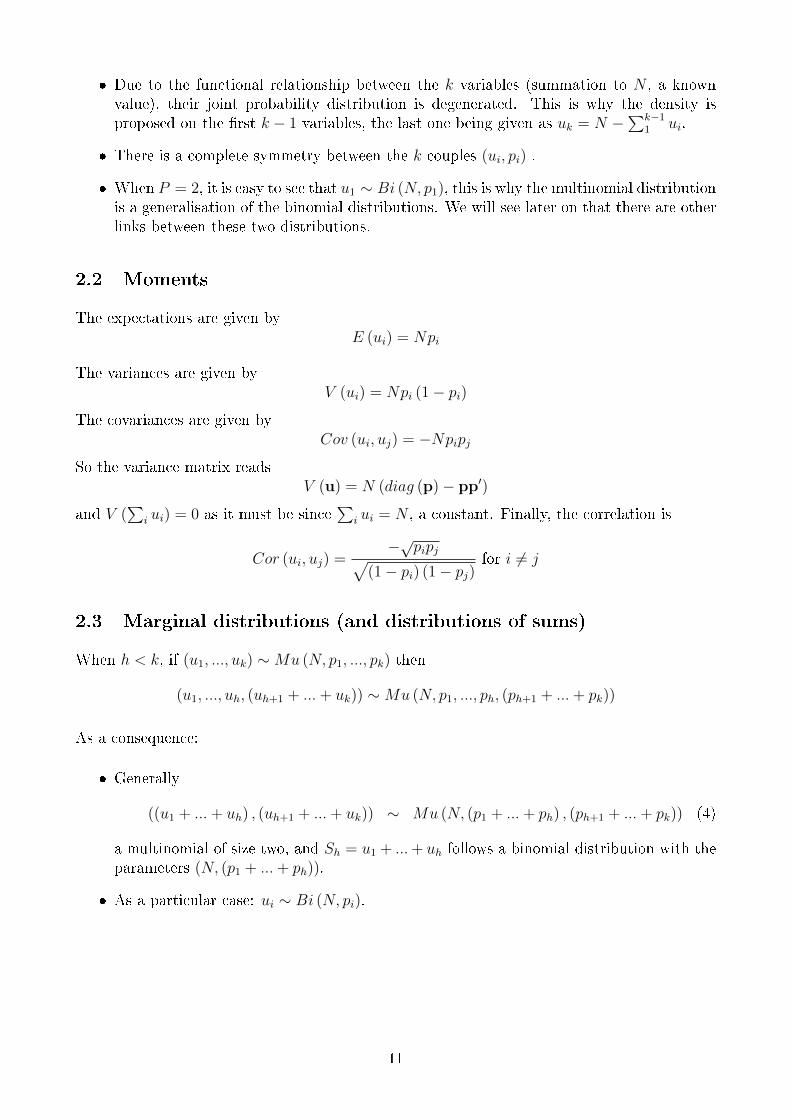
� Due to the functional relationship between the k variables (summation to N , a knownvalue), their joint probability distribution is degenerated. This is why the density isproposed on the �rst k − 1 variables, the last one being given as uk = N −

∑k−11 ui.

� There is a complete symmetry between the k couples (ui, pi) .

� When P = 2, it is easy to see that u1 ∼ Bi (N, p1), this is why the multinomial distributionis a generalisation of the binomial distributions. We will see later on that there are otherlinks between these two distributions.

2.2 Moments

The expectations are given byE (ui) = Npi

The variances are given byV (ui) = Npi (1− pi)

The covariances are given byCov (ui, uj) = −Npipj

So the variance matrix readsV (u) = N (diag (p)− pp′)

and V (∑

i ui) = 0 as it must be since∑

i ui = N , a constant. Finally, the correlation is

Cor (ui, uj) =−√pipj√

(1− pi) (1− pj)for i 6= j

2.3 Marginal distributions (and distributions of sums)

When h < k, if (u1, ..., uk) ∼Mu (N, p1, ..., pk) then

(u1, ..., uh, (uh+1 + ...+ uk)) ∼Mu (N, p1, ..., ph, (ph+1 + ...+ pk))

As a consequence:

� Generally

((u1 + ...+ uh) , (uh+1 + ...+ uk)) ∼ Mu (N, (p1 + ...+ ph) , (ph+1 + ...+ pk)) (4)

a multinomial of size two, and Sh = u1 + ...+ uh follows a binomial distribution with theparameters (N, (p1 + ...+ ph)).

� As a particular case: ui ∼ Bi (N, pi).

11

2.4 Conditional distributions

When h < k, if (u1, ..., uk) ∼Mu (N, p1, ..., pk) then

((u1, ..., uh) | uh+1, ..., uk) ∼Mu

(N −

k∑i=h+1

ui,p1∑hi=1 pi

, ...,ph∑hi=1 pi

)(5)

An important consequence of this formulae is that (u1, ..., uh) depends on (uh+1, ..., uk) onlythrough their sum, (uh+1 + ...+ uk). From this, it is not di�cult to see that when g < h:(

g∑i=1

ui |h∑i=1

ui

)∼ Bi

(h∑i=1

ui,

∑gi=1 pi∑hi=1 pi

)(6)

It can also be shown that u1, (u2 | u1) , (u3 | u1 + u2) , ..., (uk−1 | u1 + ...+ uk−2) are independentand follow binomial distributions:(

uj |j−1∑u=1

uu

)∼ Bi

(N −

j−1∑u=1

uu,pj

1−∑j−1

u=1 pu

). (7)

2.5 Construction

2.5.1 With independent Poisson distributions

Let wi, i = 1, ..., k a series of independently distributed Po (λi) variables, then(w1, ..., wk |

k∑i=1

wi = N

)∼Mu

(N,

λ1∑ki=1 λi

, ...,λk∑ki=1 λi

).

So the (ui) can be seen as a set of Poisson variables constrained to sum to N and havingparameters proportional to the probabilities pi.

Notice that this kind of condition (the sum be equal to a given value) is not a�ordable withbugs softwares.

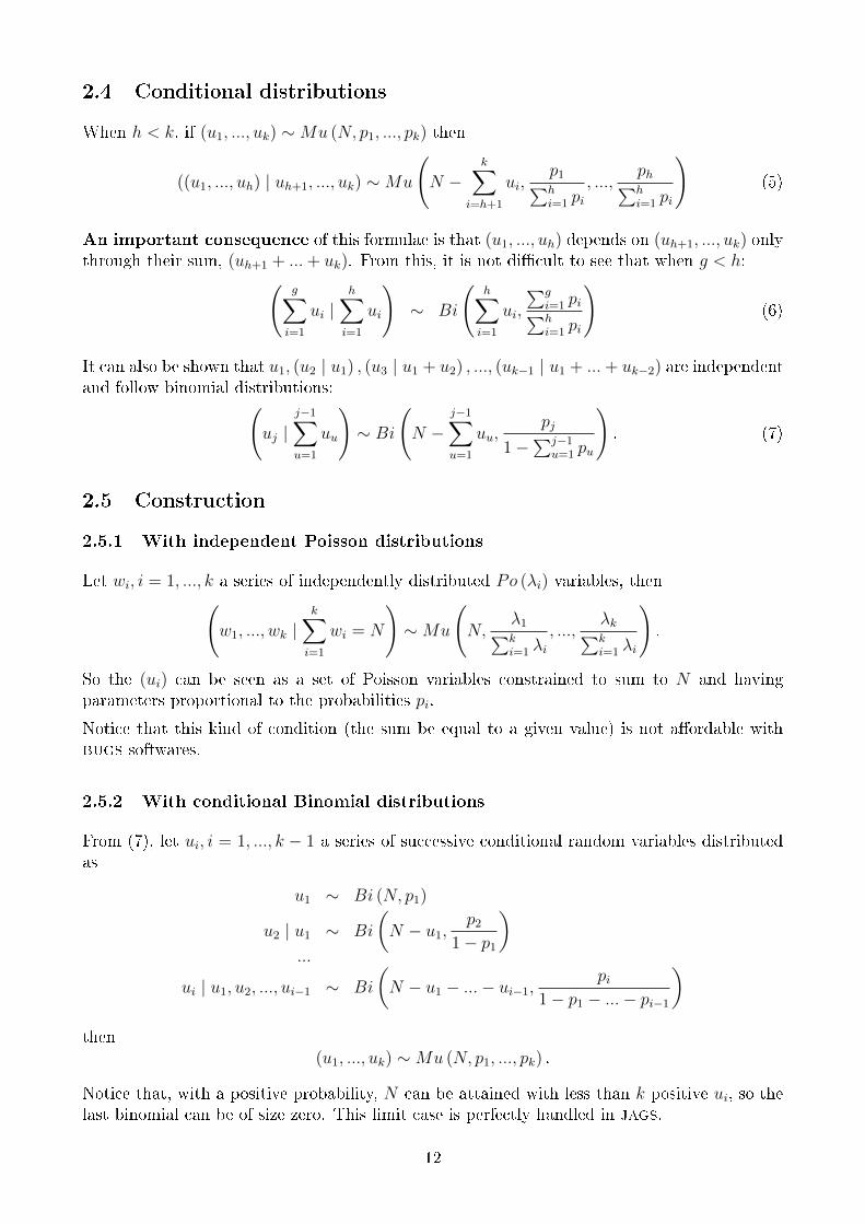
2.5.2 With conditional Binomial distributions

From (7), let ui, i = 1, ..., k − 1 a series of successive conditional random variables distributedas

u1 ∼ Bi (N, p1)

u2 | u1 ∼ Bi

(N − u1,

p2

1− p1

)...

ui | u1, u2, ..., ui−1 ∼ Bi

(N − u1 − ...− ui−1,

pi1− p1 − ...− pi−1

)then

(u1, ..., uk) ∼Mu (N, p1, ..., pk) .

Notice that, with a positive probability, N can be attained with less than k positive ui, so thelast binomial can be of size zero. This limit case is perfectly handled in jags.

12

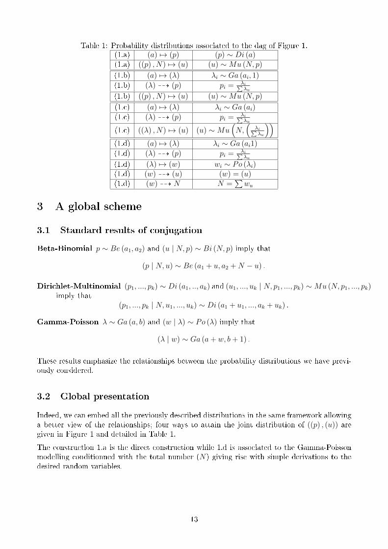
Table 1: Probability distributions associated to the dag of Figure 1.(1.a) (a) 7→ (p) (p) ∼ Di (a)(1.a) ((p) , N) 7→ (u) (u) ∼Mu (N, p)

(1.b) (a) 7→ (λ) λi ∼ Ga (ai, 1)

(1.b) (λ) 99K (p) pi =λi∑λu

(1.b) ((p) , N) 7→ (u) (u) ∼Mu (N, p)

(1.c) (a) 7→ (λ) λi ∼ Ga (ai)

(1.c) (λ) 99K (p) pi =λi∑λu

(1.c) ((λ) , N) 7→ (u) (u) ∼Mu(N,(

λi∑λu

))(1.d) (a) 7→ (λ) λi ∼ Ga (ai1)

(1.d) (λ) 99K (p) pi =λi∑λu

(1.d) (λ) 7→ (w) wi ∼ Po (λi)(1.d) (w) 99K (u) (w) = (u)(1.d) (w) 99K N N =

∑wu

3 A global scheme

3.1 Standard results of conjugation

Beta-Binomial p ∼ Be (a1, a2) and (u | N, p) ∼ Bi (N, p) imply that

(p | N, u) ∼ Be (a1 + u, a2 +N − u) .

Dirichlet-Multinomial (p1, ..., pk) ∼ Di (a1, .., ak) and (u1, ..., uk | N, p1, ..., pk) ∼Mu (N, p1, ..., pk)imply that

(p1, ..., pk | N, u1, ..., uk) ∼ Di (a1 + u1, ..., ak + uk) .

Gamma-Poisson λ ∼ Ga (a, b) and (w | λ) ∼ Po (λ) imply that

(λ | w) ∼ Ga (a+ w, b+ 1) .

These results emphasize the relationships between the probability distributions we have previ-ously considered.

3.2 Global presentation

Indeed, we can embed all the previously described distributions in the same framework allowinga better view of the relationships; four ways to attain the joint distribution of ((p) , (u)) aregiven in Figure 1 and detailed in Table 1.

The construction 1.a is the direct construction while 1.d is associated to the Gamma-Poissonmodelling conditionned with the total number (N) giving rise with simple derivations to thedesired random variables.

13

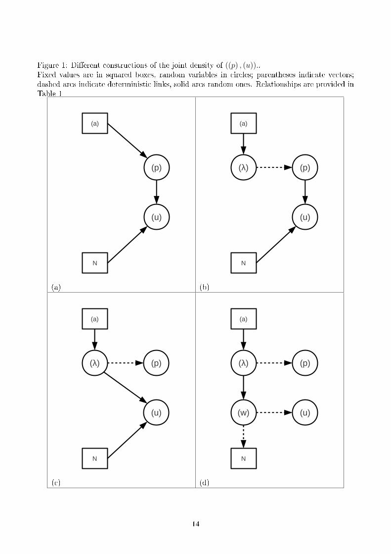
Figure 1: Di�erent constructions of the joint density of ((p) , (u))..Fixed values are in squared boxes, random variables in circles; parentheses indicate vectors;dashed arcs indicate deterministic links, solid arcs random ones. Relationships are provided inTable 1

(a)

(p)

(u)

N

(a)

(b)

(λ) (p)

(u)

N

(a)

(c)

(λ) (p)

(u)

N

(a)

(d)

(λ)

(w)

(p)

(u)

N

(a)

14

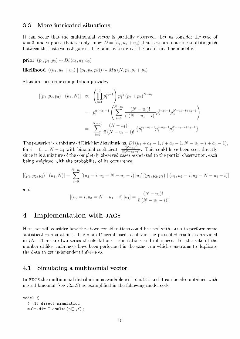
3.3 More intricated situations

It can occur that the multinomial vector is partially observed. Let us consider the case ofk = 3, and suppose that we only know D = (u1, u2 + u3) that is we are not able to distinguishbetween the last two categories. The point is to derive the posterior. The model is :

prior (p1, p2, p3) ∼ Di (a1, a2, a3)

likelihood ((u1, u2 + u3) | (p1, p2, p3)) ∼Mu (N, p1, p2 + p3)

Standard posterior computation provides

[(p1, p2, p3) | (u1, N)] ∝

(3∏i=1

pai−1i

)pu11 (p2 + p3)

N−u1

= pu1+a1−11

(N−u1∑i=0

(N − u1)!

i! (N − u1 − i)!pi+a2−1

2 pN−u1−i+a3−13

)

=

N−u1∑i=0

(N − u1)!

i! (N − u1 − i)!{pu1+a1−1

1 pi+a2−12 pN−u1−i+a3−1

3

}The posterior is a mixture of Dirichlet distributions,Di (u1 + a1 − 1, i+ a2 − 1, N − u1 − i+ a3 − 1),

for i = 0, ..., N − u1 with binomial coe�cients (N−u1)!i!(N−u1−i)! . This could have been seen directly

since it is a mixture of the completely observed cases associated to the partial observation, eachbeing weighted with the probability of its occurrence:

[(p1, p2, p3) | (u1, N)] =

N−u1∑i=0

[(u2 = i, u3 = N − u1 − i) |u1] [(p1, p2, p3) | (u1, u2 = i, u3 = N − u1 − i)]

and

[(u2 = i, u3 = N − u1 − i) |u1] =(N − u1)!

i! (N − u1 − i)!.

4 Implementation with jags

Here, we will consider how the above considerations could be used with jags to perform somestatistical computations. The main R script used to obtain the presented results is providedin �A. There are two series of calculations : simulations and inferences. For the sake of thenumber of �les, inferences have been performed in the same run which constrains to duplicatethe data to get independent inferences.

4.1 Simulating a multinomial vector

In bugs the multinomial distribution is available with dmulti and it can be also obtained withnested binomial (see �2.5.2) as exampli�ed in the following model code.

model {

# (1) direct simulation

mult.dir ~ dmulti(p[],N);

15

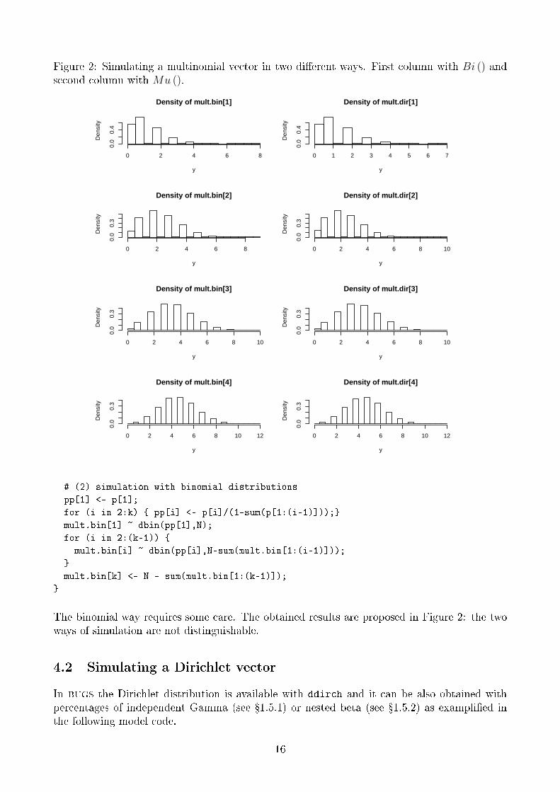
Figure 2: Simulating a multinomial vector in two di�erent ways. First column with Bi () andsecond column with Mu ().

y

Den

sity

0 2 4 6 8

0.0

0.4

Density of mult.bin[1]

y

Den

sity

0 2 4 6 8

0.0

0.3


y

Den

sity

0 2 4 6 8 10

0.0

0.3


y

Den

sity

0 2 4 6 8 10 12

0.0

0.3


y

Den

sity

0 1 2 3 4 5 6 7

0.0

0.4

Density of mult.dir[1]

y

Den

sity

0 2 4 6 8 10

0.0

0.3


y

Den

sity

0 2 4 6 8 10

0.0

0.3


y

Den

sity

0 2 4 6 8 10 12

0.0

0.3


# (2) simulation with binomial distributions

pp[1] <- p[1];

for (i in 2:k) { pp[i] <- p[i]/(1-sum(p[1:(i-1)]));}

mult.bin[1] ~ dbin(pp[1],N);

for (i in 2:(k-1)) {

mult.bin[i] ~ dbin(pp[i],N-sum(mult.bin[1:(i-1)]));

}

mult.bin[k] <- N - sum(mult.bin[1:(k-1)]);

}

The binomial way requires some care. The obtained results are proposed in Figure 2: the twoways of simulation are not distinguishable.

4.2 Simulating a Dirichlet vector

In bugs the Dirichlet distribution is available with ddirch and it can be also obtained withpercentages of independent Gamma (see �1.5.1) or nested beta (see �1.5.2) as exampli�ed inthe following model code.

16

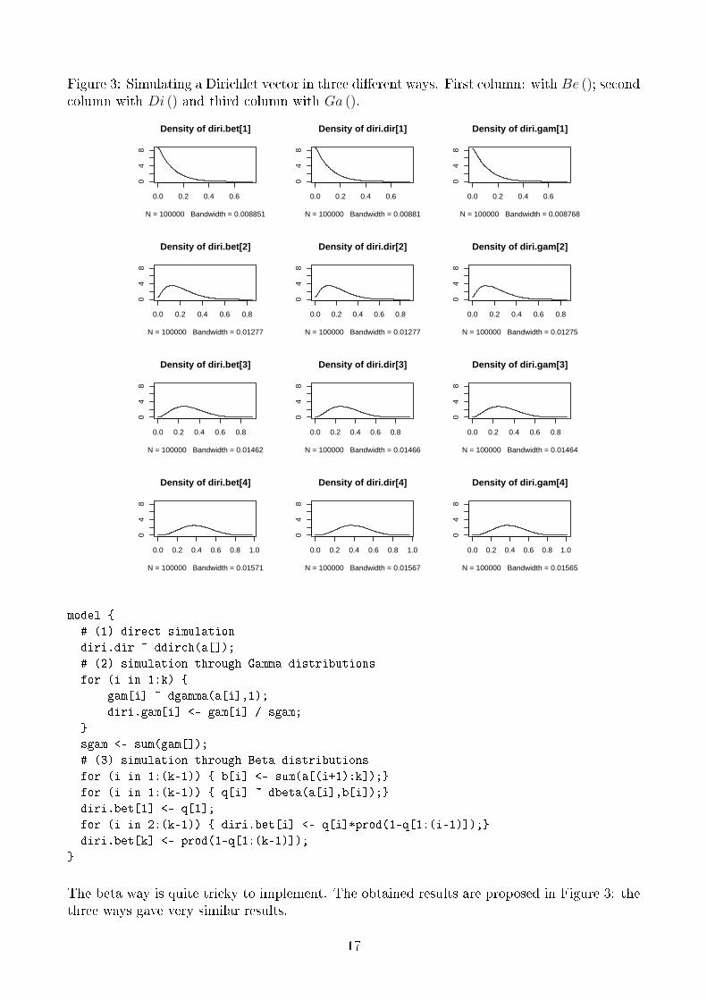
Figure 3: Simulating a Dirichlet vector in three di�erent ways. First column: with Be (); secondcolumn with Di () and third column with Ga ().

0.0 0.2 0.4 0.6

04

8

N = 100000 Bandwidth = 0.008851

Density of diri.bet[1]

0.0 0.2 0.4 0.6 0.8

04

8

N = 100000 Bandwidth = 0.01277


0.0 0.2 0.4 0.6 0.8

04

8

N = 100000 Bandwidth = 0.01462


0.0 0.2 0.4 0.6 0.8 1.0

04

8

N = 100000 Bandwidth = 0.01571


0.0 0.2 0.4 0.6

04

8

N = 100000 Bandwidth = 0.00881

Density of diri.dir[1]

0.0 0.2 0.4 0.6 0.8

04

8

N = 100000 Bandwidth = 0.01277


0.0 0.2 0.4 0.6 0.8

04

8

N = 100000 Bandwidth = 0.01466


0.0 0.2 0.4 0.6 0.8 1.0

04

8

N = 100000 Bandwidth = 0.01567


0.0 0.2 0.4 0.6

04

8

N = 100000 Bandwidth = 0.008768

Density of diri.gam[1]

0.0 0.2 0.4 0.6 0.8

04

8

N = 100000 Bandwidth = 0.01275


0.0 0.2 0.4 0.6 0.8

04

8N = 100000 Bandwidth = 0.01464


0.0 0.2 0.4 0.6 0.8 1.0

04

8

N = 100000 Bandwidth = 0.01565


model {

# (1) direct simulation

diri.dir ~ ddirch(a[]);

# (2) simulation through Gamma distributions

for (i in 1:k) {

gam[i] ~ dgamma(a[i],1);

diri.gam[i] <- gam[i] / sgam;

}

sgam <- sum(gam[]);

# (3) simulation through Beta distributions

for (i in 1:(k-1)) { b[i] <- sum(a[(i+1):k]);}

for (i in 1:(k-1)) { q[i] ~ dbeta(a[i],b[i]);}

diri.bet[1] <- q[1];

for (i in 2:(k-1)) { diri.bet[i] <- q[i]*prod(1-q[1:(i-1)]);}

diri.bet[k] <- prod(1-q[1:(k-1)]);

}

The beta way is quite tricky to implement. The obtained results are proposed in Figure 3: thethree ways gave very similar results.

17

4.3 Inferring from multinomial vectors with �xed sizes

Using the di�erent ways of simulating multinomial distributions, ones can try some inferenceabout the probability parameter when some multinomial data have been observed. Here is theproposed bugs model when the size of the multinomial is considered as �xed.

model {

# (0) prior on the probabilities

p1 ~ ddirch(a[]); p2 ~ ddirch(a[]);

# (1) inference with dmult

for (ii in 1:nbds) { YY1[ii,] ~ dmulti(p1[],nb[ii]);}

# (2) inference with dbin

pp[1] <- p2[1];

for (i in 2:k) { pp[i] <- p2[i]/(1-sum(p2[1:(i-1)]));}

for (ii in 1:nbds) {

YY2[ii,1] ~ dbin(pp[1],nb[ii]);

for (jj in 2:(k-1)) {

YY2[ii,jj] ~ dbin(pp[jj],nb[ii]-sum(YY2[ii,1:(jj-1)]));

}

}

}

Results are graphically presented in Figure 4. The posterior distributions looks identical.

4.4 Inferring from multinomial vectors with random sizes

The same exercice can be made when the size of the multinomial data is supposed random(not been monitored by the experimenter). To do so, to comply bugs requirements, the sizesare duplicated to give direct likelihood to the multinomial vectors and to the sizes; this has noconsequence on the statistical analysis as far as no stochastic dependence is introduced betweenthe parameter of the two parts.

We will distinguish two cases because the results are di�erent.

4.4.1 Every multinomial has got a non null size

Here is the bugs model code.

model {

# (0.a) prior on the parameters

p1 ~ ddirch(a[]); p2 ~ ddirch(a[]);

lambda1 ~ dunif(lin,lax); lambda2 ~ dunif(lin,lax);

# (0.b) likelihood of the sizes

for (ii in 1:nbds) { nb1[ii] ~ dpois(lambda1);}

for (ii in 1:nbds) { nb2[ii] ~ dpois(lambda2);}

# (1) inference with dmulti

for (ii in 1:nbds) { YY1[ii,] ~ dmulti(p1[],nb1[ii]);}

# (1) inference with dbin

pp[1] <- p2[1];


18

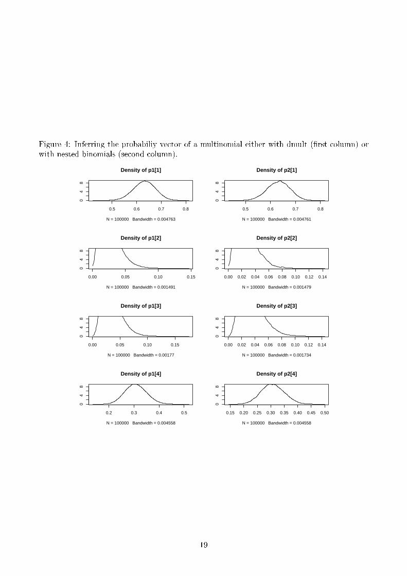
Figure 4: Inferring the probabiliy vector of a multinomial either with dmult (�rst column) orwith nested binomials (second column).

0.5 0.6 0.7 0.8

04

8

N = 100000 Bandwidth = 0.004763

Density of p1[1]

0.00 0.05 0.10 0.15

04

8

N = 100000 Bandwidth = 0.001491

Density of p1[2]

0.00 0.05 0.10 0.15

04

8

N = 100000 Bandwidth = 0.00177

Density of p1[3]

0.2 0.3 0.4 0.5

04

8

N = 100000 Bandwidth = 0.004558

Density of p1[4]

0.5 0.6 0.7 0.8

04

8N = 100000 Bandwidth = 0.004761

Density of p2[1]

0.00 0.02 0.04 0.06 0.08 0.10 0.12 0.14

04

8

N = 100000 Bandwidth = 0.001479

Density of p2[2]

0.00 0.02 0.04 0.06 0.08 0.10 0.12 0.14

04

8

N = 100000 Bandwidth = 0.001734

Density of p2[3]

0.15 0.20 0.25 0.30 0.35 0.40 0.45 0.50

04

8

N = 100000 Bandwidth = 0.004558

Density of p2[4]

19

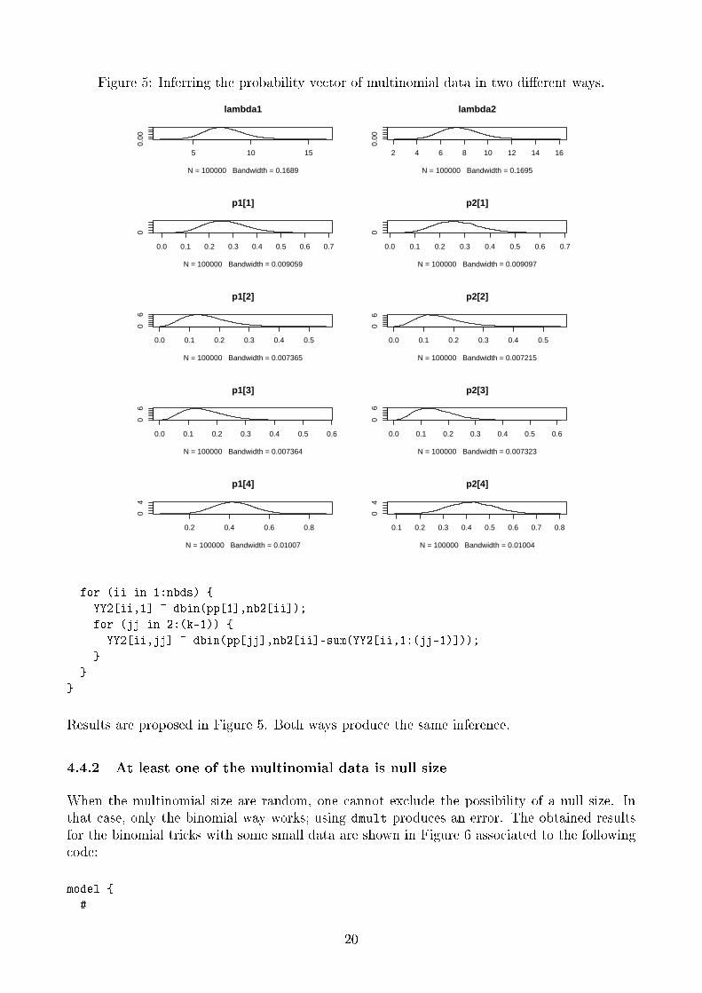
Figure 5: Inferring the probability vector of multinomial data in two di�erent ways.

5 10 15

0.00

lambda1

N = 100000 Bandwidth = 0.1689

0.0 0.1 0.2 0.3 0.4 0.5 0.6 0.7

0

p1[1]

N = 100000 Bandwidth = 0.009059

0.0 0.1 0.2 0.3 0.4 0.5

06

p1[2]

N = 100000 Bandwidth = 0.007365

0.0 0.1 0.2 0.3 0.4 0.5 0.6

06

p1[3]

N = 100000 Bandwidth = 0.007364

0.2 0.4 0.6 0.8

04

p1[4]

N = 100000 Bandwidth = 0.01007

2 4 6 8 10 12 14 16

0.00

lambda2

N = 100000 Bandwidth = 0.1695

0.0 0.1 0.2 0.3 0.4 0.5 0.6 0.7

0

p2[1]

N = 100000 Bandwidth = 0.009097

0.0 0.1 0.2 0.3 0.4 0.5

06

p2[2]

N = 100000 Bandwidth = 0.007215

0.0 0.1 0.2 0.3 0.4 0.5 0.6

06

p2[3]

N = 100000 Bandwidth = 0.007323

0.1 0.2 0.3 0.4 0.5 0.6 0.7 0.8

04

p2[4]

N = 100000 Bandwidth = 0.01004


YY2[ii,1] ~ dbin(pp[1],nb2[ii]);

for (jj in 2:(k-1)) {

YY2[ii,jj] ~ dbin(pp[jj],nb2[ii]-sum(YY2[ii,1:(jj-1)]));

}

}

}

Results are proposed in Figure 5. Both ways produce the same inference.

4.4.2 At least one of the multinomial data is null size

When the multinomial size are random, one cannot exclude the possibility of a null size. Inthat case, only the binomial way works; using dmult produces an error. The obtained resultsfor the binomial tricks with some small data are shown in Figure 6 associated to the followingcode:

model {

#

20

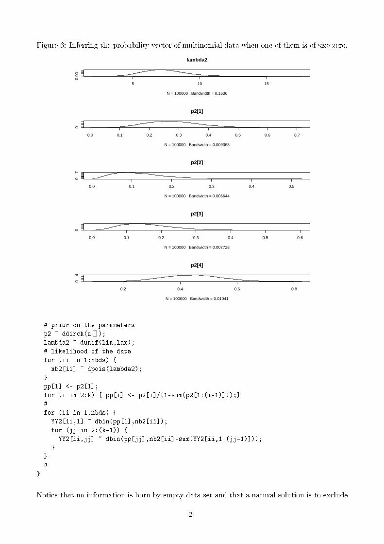
Figure 6: Inferring the probability vector of multinomial data when one of them is of size zero.

5 10 15

0.00

lambda2

N = 100000 Bandwidth = 0.1636

0.0 0.1 0.2 0.3 0.4 0.5 0.6 0.7

0

p2[1]

N = 100000 Bandwidth = 0.009368

0.0 0.1 0.2 0.3 0.4 0.5

07

p2[2]

N = 100000 Bandwidth = 0.006644

0.0 0.1 0.2 0.3 0.4 0.5 0.6

0

p2[3]

N = 100000 Bandwidth = 0.007728

0.2 0.4 0.6 0.8

04

p2[4]

N = 100000 Bandwidth = 0.01041

# prior on the parameters

p2 ~ ddirch(a[]);

lambda2 ~ dunif(lin,lax);

# likelihood of the data


nb2[ii] ~ dpois(lambda2);

}

pp[1] <- p2[1];


#


YY2[ii,1] ~ dbin(pp[1],nb2[ii]);

for (jj in 2:(k-1)) {

YY2[ii,jj] ~ dbin(pp[jj],nb2[ii]-sum(YY2[ii,1:(jj-1)]));

}

}

#

}

Notice that no information is born by empty data set and that a natural solution is to exclude

21

them from the statistical analysis, making the dmult solution always available.

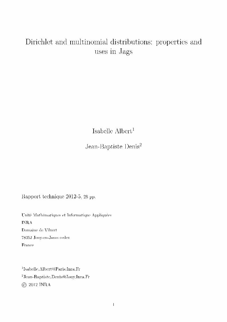
4.5 Inferring from a Dirichlet vector

Even if not a so frequent situation, we can check what occurs when the observations are atthe level of the Dirichlet variables. This implies an additional level in the model to focus theinference on the a parameter. An example is given in the following bugsmodel code consideringthe three identi�ed ways : (i) the direct ddirch use, (iii) the dbeta construction theoriticallyexact and (iii) a dgamma approximation.

The dbeta construction implies the computation of qi, direct transformations of the observedpi (see �1.5.2) and the code in the Appendix for the details.

The dgamma construction is only an approximation. There is no way for a transformation of theobservations as done for the dbeta construction6. Here the parameterization of the gammasvariables is de�ned such that their expectations and variances be equal to those of a Dirichletvector, forgetting the existing covariance of (1). More precisely, with the notations of �1.1 andthe de�nition of gamma distributions in Footnote 4 we use

Ga

(ai (1 + A)

A− ai,A (1 + A)

A− ai

)for the ith probability. Higher will be the dimension k of the Dirichlet, better we can imaginewill be the approximation.

model {

# (0) priors

for (ii in 1:k) {

a1[ii] ~ dunif(lin,lax);



}

# (1) likelihood with dirichlet

p1 ~ ddirch(a1[]);

# (2) likelihood with betas

for (i in 1:(k-1)) {

b[i] <- sum(a2[(i+1):k]);

q2[i] ~ dbeta(a2[i],b[i]);

}

# (3) likelihood with gammas

A <- sum(a3[]);

for (i in 1:k) {

p3[i] ~ dgamma(a3[i]*(1+A)/(A-a3[i]),

A*(1+A)/(A-a3[i]));

}

}

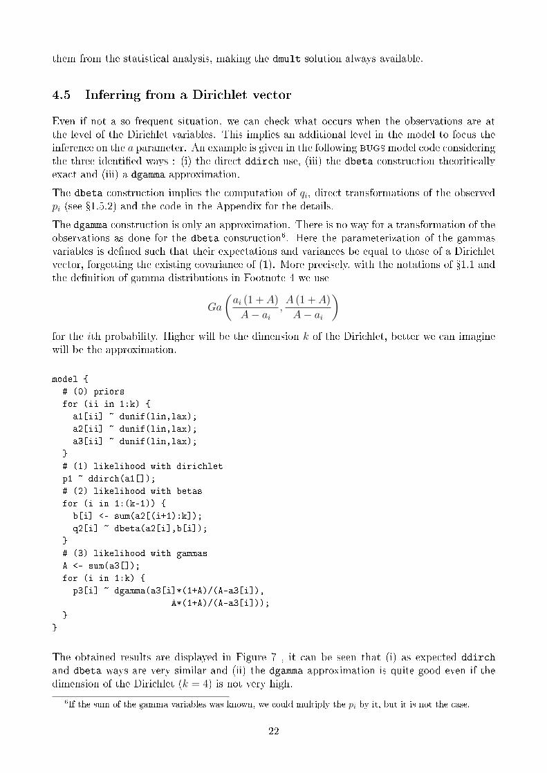
The obtained results are displayed in Figure 7 , it can be seen that (i) as expected ddirch

and dbeta ways are very similar and (ii) the dgamma approximation is quite good even if thedimension of the Dirichlet (k = 4) is not very high.

6If the sum of the gamma variables was known, we could multiply the pi by it, but it is not the case.

22

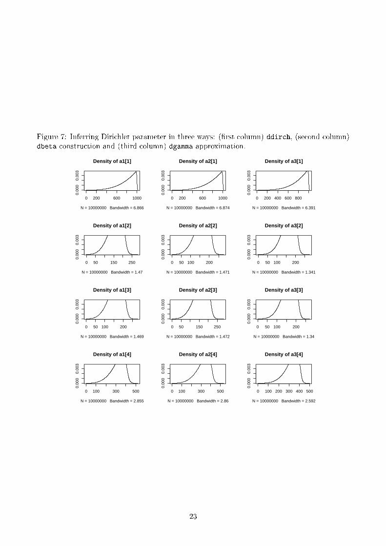
Figure 7: Inferring Dirichlet parameter in three ways: (�rst column) ddirch, (second column)dbeta construction and (third column) dgamma approximation.

0 200 600 1000

0.00

00.

003

N = 10000000 Bandwidth = 6.866

Density of a1[1]

0 50 150 250

0.00

00.

003

N = 10000000 Bandwidth = 1.47

Density of a1[2]

0 50 100 200

0.00

00.

003

N = 10000000 Bandwidth = 1.469

Density of a1[3]

0 100 300 500

0.00

00.

003

N = 10000000 Bandwidth = 2.855

Density of a1[4]

0 200 600 1000

0.00

00.

003

N = 10000000 Bandwidth = 6.874

Density of a2[1]

0 50 100 200

0.00

00.

003

N = 10000000 Bandwidth = 1.471

Density of a2[2]

0 50 150 250

0.00

00.

003

N = 10000000 Bandwidth = 1.472

Density of a2[3]

0 100 300 500

0.00

00.

003

N = 10000000 Bandwidth = 2.86

Density of a2[4]

0 200 400 600 800

0.00

00.

003

N = 10000000 Bandwidth = 6.391

Density of a3[1]

0 50 100 200

0.00

00.

003

N = 10000000 Bandwidth = 1.341

Density of a3[2]

0 50 100 200

0.00

00.

003

N = 10000000 Bandwidth = 1.34

Density of a3[3]

0 100 200 300 400 500

0.00

00.

003

N = 10000000 Bandwidth = 2.592

Density of a3[4]

23

References

The most complete derivations were found in Johnson and Kotz, Distribution in Statistics:Continuous Multivariate Distributions (1972, John Wiley) �40.5, pages 231-235.

It is also of interest to consult some articles of the Wikipedia, for instancehttp://en.wikipedia.org/wiki/Neutral_vector.

Jags is a similar software toWinBugs available at http://www-�s.iarc.fr/~martyn/software/jags/.Contrary to WinBugs, it can be run under Linux (an also MSWindows). It has got extendedfacilities as vector/matrix/array de�nition of the nodes (to avoid loops).

A Main R script

Here is the complete R script used for all calculations related to �4. The called �les to describethe model were given in the text above: dirimul.mulsim.jam in �4.1, dirimul.dirsim.jam in�4.2, dirimul.mulinf1.jam in �4.3, dirimul.mulinf2.jam in �4.4.1, dirimul.mulinf3.jamin �4.4.2 and dirimul.dirinf1.jam in �4.5,

# 12_06_06 12_06_07 12_06_20 12_06_21 12_07_18

library(rjags)

# initialization

nbsimu <- 100000; nbburnin <- 10000;

#nbsimu <- 1000; nbburnin <- 100;

files <- TRUE;

fitext <- "dirimul.res.txt";

if (files) { sink(fitext); sink();}

fifi <- function(nom) {

res <- rep(NA,2);

res[1] <- paste("dirimul",nom,"jam",sep=".");

res[2] <- paste("dirimul",nom,"pdf",sep=".");

res;

}

# Simulating a multinomial vector

".RNG.state" <- c(19900, 14957, 25769);

set.seed(1234);

nom <- "mulsim"; ff <- fifi(nom);

p <- 1:4/sum(1:4);

k <- length(p);

N <- 12;

tomonitor <- c("mult.dir","mult.bin");

constants <- list(p=p,k=k,N=N);

modele <- jags.model(file=ff[1],data=constants);

update(modele,10);

resultats <- coda.samples(modele,tomonitor,n.iter=nbsimu);

if (files) {

sink(fitext,append=TRUE);

cat("\n\n\n",nom,"\n\n");

}

24

print(summary(resultats));

if (files) { sink();}

if (files) { pdf(ff[2]);}

par(mfcol=c(4,2));

densplot(resultats,show.obs=FALSE);

if (files) { dev.off();}

cat(nom,": <Enter> to continue\n");

if (!files) { scan();}

# Simulating a Dirichlet vector

".RNG.state" <- c(19900, 14957, 25769);

set.seed(1234);

nom <- "dirsim"; ff <- fifi(nom);

a <- 1:4;

k <- length(a);

tomonitor <- c("diri.dir","diri.gam","diri.bet");

constants <- list(a=a,k=k);


update(modele,10);


if (files) {



}




par(mfcol=c(4,3));





# Inferring multinomial vectors of fixed sizes

".RNG.state" <- c(19900, 14957, 25769);

set.seed(1234);

nom <- "mulinf1"; ff <- fifi(nom);

a <- rep(1,4);

k <- length(a);

tomonitor <- c("p1","p2");

YY1 <- matrix(c(1,0,2,7,

70,2,1,27),byrow=TRUE,2,k);

nbds <- nrow(YY1);

nb <- apply(YY1,1,sum);

YY2 <- YY1;

if (files) {



}

print(YY1);


constants <- list(a=a,k=k,nbds=nbds,nb=nb,

25

YY1=YY1,YY2=YY2);


update(modele,nbburnin);


if (files) {



}




par(mfcol=c(4,2));





# Inferring multinomial vectors with positive random sizes

".RNG.state" <- c(19900, 14957, 25769);

set.seed(1234);


a <- rep(1,4);

k <- length(a);

lin <- 1; lax <- 100;

tomonitor <- c("p1","lambda1","p2","lambda2");

YY1 <- matrix(c(1,0,2,7,

0,1,0,0,

5,2,1,3),byrow=TRUE,3,k);

nbds <- nrow(YY1);

nb1 <- apply(YY1,1,sum);

YY2 <- YY1; nb2 <- nb1;

if (files) {



}

print(YY1);


constants <- list(a=a,k=k,nbds=nbds,lin=lin,lax=lax,

nb1=nb1,YY1=YY1,nb2=nb2,YY2=YY2

);




if (files) {



}




par(mfcol=c(5,2));

for (ip in c(1,3:6,2,7:10)) {

26

densplot(resultats[[1]][,ip],show.obs=FALSE,

main=dimnames(resultats[[1]])[[2]][ip]);

}




# Inferring multinomial vectors with positive and nought random sizes

".RNG.state" <- c(19900, 14957, 25769);

set.seed(1234);


a <- rep(1,4);

k <- length(a);

lin <- 1; lax <- 100;

tomonitor <- c("p2","lambda2");

YY1 <- matrix(c(1,0,2,7,

0,0,0,0,

5,2,1,3),byrow=TRUE,3,k);

nbds <- nrow(YY1);

nb1 <- apply(YY1,1,sum);

YY2 <- YY1; nb2 <- nb1;

if (files) {



}

print(YY1);


constants <- list(a=a,k=k,nbds=nbds,lin=lin,lax=lax,

nb2=nb2,YY2=YY2

);




if (files) {



}




par(mfcol=c(5,1));

for (ip in 1:5) {

densplot(resultats[[1]][,ip],show.obs=FALSE,

main=dimnames(resultats[[1]])[[2]][ip]);

}




# Inferring Dirichlet vectors

".RNG.state" <- c(19900, 14957, 25769);

set.seed(1234);

27

nom <- "dirinf1"; ff <- fifi(nom);

p <- c(5,1,1,2);

k <- length(p);

lin <- 1; lax <- 1000;

tomonitor <- c("a1","a2","a3");

p <- p/sum(p);

p1 <- p2 <- p3 <- p;

q2 <- p2[-4];

q2[2] <- q2[2]/(1-q2[1]);

q2[3] <- q2[3]/(1-q2[1])/(1-q2[2]);

constants <- list(k=k,lin=lin,lax=lax,p1=p1,q2=q2,p3=p3);


update(modele,nbburnin*100);

resultats <- coda.samples(modele,tomonitor,n.iter=nbsimu*100);

if (files) {



}




par(mfcol=c(4,3));





# The end

cat("C'est FINI !\n");

28